Cut and Tag QC
Steven Yu
2025-07-01
Last updated: 2026-01-15
Checks: 7 0
Knit directory: DXR_continue/
This reproducible R Markdown analysis was created with workflowr (version 1.7.1). The Checks tab describes the reproducibility checks that were applied when the results were created. The Past versions tab lists the development history.
Great! Since the R Markdown file has been committed to the Git repository, you know the exact version of the code that produced these results.
Great job! The global environment was empty. Objects defined in the global environment can affect the analysis in your R Markdown file in unknown ways. For reproduciblity it’s best to always run the code in an empty environment.
The command set.seed(20250701) was run prior to running
the code in the R Markdown file. Setting a seed ensures that any results
that rely on randomness, e.g. subsampling or permutations, are
reproducible.
Great job! Recording the operating system, R version, and package versions is critical for reproducibility.
Nice! There were no cached chunks for this analysis, so you can be confident that you successfully produced the results during this run.
Great job! Using relative paths to the files within your workflowr project makes it easier to run your code on other machines.
Great! You are using Git for version control. Tracking code development and connecting the code version to the results is critical for reproducibility.
The results in this page were generated with repository version e59970a. See the Past versions tab to see a history of the changes made to the R Markdown and HTML files.
Note that you need to be careful to ensure that all relevant files for
the analysis have been committed to Git prior to generating the results
(you can use wflow_publish or
wflow_git_commit). workflowr only checks the R Markdown
file, but you know if there are other scripts or data files that it
depends on. Below is the status of the Git repository when the results
were generated:
Ignored files:
    Ignored:    .Rhistory
    Ignored:    .Rproj.user/
    Ignored:    data/Bed_exports/
    Ignored:    data/Cormotif_data/
    Ignored:    data/DER_data/
    Ignored:    data/Other_paper_data/
    Ignored:    data/RDS_files/
    Ignored:    data/TE_annotation/
    Ignored:    data/alignment_summary.txt
    Ignored:    data/all_peak_final_dataframe.txt
    Ignored:    data/cell_line_info_.tsv
    Ignored:    data/full_summary_QC_metrics.txt
    Ignored:    data/motif_lists/
    Ignored:    data/number_frag_peaks_summary.txt

Untracked files:
    Untracked:  H3K27ac_all_regions_test.bed
    Untracked:  H3K27ac_consensus_clusters_test.bed
    Untracked:  analysis/GREAT_H3K27ac.Rmd
    Untracked:  analysis/Top2a_Top2b_expression.Rmd
    Untracked:  analysis/chromHMM.Rmd
    Untracked:  analysis/human_genome_composition.Rmd
    Untracked:  analysis/maps_and_plots.Rmd
    Untracked:  analysis/proteomics.Rmd
    Untracked:  other_analysis/

Unstaged changes:
    Modified:   analysis/H3K9me3_summit_processing.Rmd
    Modified:   analysis/Motif_cluster_analysis.Rmd
    Modified:   analysis/Outlier_removal.Rmd
    Modified:   analysis/final_analysis.Rmd
    Modified:   analysis/summit_files_processing.Rmd
Note that any generated files, e.g. HTML, png, CSS, etc., are not included in this status report because it is ok for generated content to have uncommitted changes.
These are the previous versions of the repository in which changes were
made to the R Markdown (analysis/multiQC_cut_tag.Rmd) and
HTML (docs/multiQC_cut_tag.html) files. If you’ve
configured a remote Git repository (see ?wflow_git_remote),
click on the hyperlinks in the table below to view the files as they
were in that past version.
| File | Version | Author | Date | Message |
|---|---|---|---|---|
| Rmd | e59970a | reneeisnowhere | 2026-01-15 | wflow_publish("analysis/multiQC_cut_tag.Rmd") |
| html | 60f3e0e | reneeisnowhere | 2025-09-03 | Build site. |
| Rmd | ed049ca | reneeisnowhere | 2025-09-03 | wflow_publish("analysis/multiQC_cut_tag.Rmd") |
| html | 5b7c212 | reneeisnowhere | 2025-08-20 | Build site. |
| Rmd | 4b88ecb | reneeisnowhere | 2025-08-20 | adding file save updates |
| html | aa92650 | reneeisnowhere | 2025-08-12 | Build site. |
| html | fb0c397 | reneeisnowhere | 2025-08-11 | Build site. |
| html | 6ea2087 | infurnoheat | 2025-08-01 | Build site. |
| html | 1bd95b2 | infurnoheat | 2025-07-30 | Build site. |
| Rmd | 8c0cfb9 | infurnoheat | 2025-07-30 | wflow_publish("analysis/multiQC_cut_tag.Rmd") |
| html | f296101 | infurnoheat | 2025-07-14 | Build site. |
| Rmd | 14a41b4 | infurnoheat | 2025-07-14 | wflow_publish("analysis/multiQC_cut_tag.Rmd") |
| html | 95dfc55 | infurnoheat | 2025-07-14 | Build site. |
| Rmd | b81a3e4 | infurnoheat | 2025-07-14 | wflow_publish("analysis/multiQC_cut_tag.Rmd") |
| html | d32e3b2 | infurnoheat | 2025-07-08 | Build site. |
| Rmd | ad15724 | infurnoheat | 2025-07-08 | wflow_publish("analysis/multiQC_cut_tag.Rmd") |
| html | 1152014 | infurnoheat | 2025-07-08 | Build site. |
| Rmd | 5920a66 | infurnoheat | 2025-07-08 | wflow_publish("analysis/multiQC_cut_tag.Rmd") |
| html | e3aa827 | infurnoheat | 2025-07-06 | Build site. |
| Rmd | fb62b9f | infurnoheat | 2025-07-06 | wflow_publish("analysis/multiQC_cut_tag.Rmd") |
| html | 19bd9f4 | infurnoheat | 2025-07-06 | Build site. |
| Rmd | e9cc9ab | infurnoheat | 2025-07-06 | wflow_publish("analysis/multiQC_cut_tag.Rmd") |
| html | 57a7b55 | infurnoheat | 2025-07-03 | Build site. |
| html | 4d5379f | infurnoheat | 2025-07-03 | Build site. |
| Rmd | efcdf08 | infurnoheat | 2025-07-03 | wflow_publish("analysis/multiQC_cut_tag.Rmd") |
| html | 838af68 | infurnoheat | 2025-07-02 | Build site. |
| html | 1b45520 | infurnoheat | 2025-07-02 | Build site. |
| html | 40eefb9 | infurnoheat | 2025-07-02 | Build site. |
| html | 88a419f | infurnoheat | 2025-07-02 | Build site. |
| Rmd | ca7a59c | infurnoheat | 2025-07-02 | wflow_publish("analysis/multiQC_cut_tag.Rmd") |
| html | 0644589 | infurnoheat | 2025-07-02 | Build site. |
| Rmd | 59eb78f | infurnoheat | 2025-07-02 | wflow_publish("analysis/multiQC_cut_tag.Rmd") |
Cut And Tag QC
Loading Packages
library(tidyverse)
library(readr)
library(edgeR)
library(ComplexHeatmap)
library(data.table)
library(dplyr)
library(stringr)
library(ggplot2)
library(viridis)
library(DT)
library(kableExtra)
library(genomation)
library(GenomicRanges)
library(chromVAR) ## For FRiP analysis and differential analysis
library(DESeq2) ## For differential analysis section
library(ggpubr) ## For customizing figures
library(corrplot) ## For correlation plot
library(ggpmisc)
library(gcplyr)
Data Initialization
sampleinfo <- read_delim("data/sample_info.tsv", delim = "\t")
multiqc_gene_stats_trim <- read_delim("data/multiqc_data_trim/multiqc_general_stats.txt",delim = "\t")
multiqc_fastqc_trim <- read_delim("data/multiqc_data_trim/multiqc_fastqc.txt",delim = "\t")
Functions
drug_pal <- c("#8B006D","#DF707E","#F1B72B", "#3386DD","#707031","#41B333")
pca_plot <-
  function(df,
           col_var = NULL,
           shape_var = NULL,
           title = "") {
    ggplot(df) + geom_point(aes_string(
      x = "PC1",
      y = "PC2",
      color = col_var,
      shape = shape_var
    ),
    size = 5) +
      labs(title = title, x = "PC 1", y = "PC 2") +
      scale_color_manual(values = c(
        "#8B006D",
        "#DF707E",
        "#F1B72B",
        "#3386DD",
        "#707031",
        "#41B333"
      ))
  }
pca_var_plot <- function(pca) {
  # x: class == prcomp
  pca.var <- pca$sdev ^ 2
  pca.prop <- pca.var / sum(pca.var)
  var.plot <-
    qplot(PC, prop, data = data.frame(PC = 1:length(pca.prop),
                                      prop = pca.prop)) +
    labs(title = 'Variance contributed by each PC',
         x = 'PC', y = 'Proportion of variance')
  plot(var.plot)
}

calc_pca <- function(x) {
  # Performs principal components analysis with prcomp
  # x: a sample-by-gene numeric matrix
  prcomp(x, scale. = TRUE, retx = TRUE)
}

get_regr_pval <- function(mod) {
  # Returns the p-value for the Fstatistic of a linear model
  # mod: class lm
  stopifnot(class(mod) == "lm")
  fstat <- summary(mod)$fstatistic
  pval <- 1 - pf(fstat[1], fstat[2], fstat[3])
  return(pval)
}

plot_versus_pc <- function(df, pc_num, fac) {
  # df: data.frame
  # pc_num: numeric, specific PC for plotting
  # fac: column name of df for plotting against PC
  pc_char <- paste0("PC", pc_num)
  # Calculate F-statistic p-value for linear model
  pval <- get_regr_pval(lm(df[, pc_char] ~ df[, fac]))
  if (is.numeric(df[, f])) {
    ggplot(df, aes_string(x = f, y = pc_char)) + geom_point() +
      geom_smooth(method = "lm") + labs(title = sprintf("p-val: %.2f", pval))
  } else {
    ggplot(df, aes_string(x = f, y = pc_char)) + geom_boxplot() +
      labs(title = sprintf("p-val: %.2f", pval))
  }
}
x_axis_labels = function(labels, every_nth = 1, ...) {
  axis(side = 1,
       at = seq_along(labels),
       labels = F)
  text(
    x = (seq_along(labels))[seq_len(every_nth) == 1],
    y = par("usr")[3] - 0.075 * (par("usr")[4] - par("usr")[3]),
    labels = labels[seq_len(every_nth) == 1],
    xpd = TRUE,
    ...
  )
}
Basic Stats
Data Processing
combo_trim_df <- multiqc_fastqc_trim %>%
 extract(., Sample, into = c("prefix","read"), regex= "(.+)_R(\\d+)", remove=FALSE) %>%
  mutate(read = paste0("R", read)) %>%
  left_join(., sampleinfo, by =c("prefix"="Library ID")) %>%
  left_join(., multiqc_gene_stats_trim, by = c("Sample" = "Sample")) %>%
  mutate(ind=factor(Individual, levels = c("Ind1","Ind2","Ind3","Ind4","Ind5"))) %>%
  mutate(trt=factor(Treatment, levels = c("VEH","5FU","DOX"))) %>%
  mutate(time=factor(Timepoint, levels=c("24T","24R","144R")))
combo_trim_df <- combo_trim_df[(!combo_trim_df$trt %in% "5FU"),]
Data Visualization
combo_trim_df %>%
  dplyr::filter(read=="R1") %>%
  group_by(trt, time, Histone_Mark) %>%
  tally() %>%
  ggplot(., aes(x = time, y= n))+
  geom_col(position="dodge",aes(fill=trt)) +
  facet_wrap(~Histone_Mark)+
  theme(axis.text.x=element_text(angle=90))+
  ylab("number of samples")+
  ggtitle("Breakdown of samples by mark and trt-time")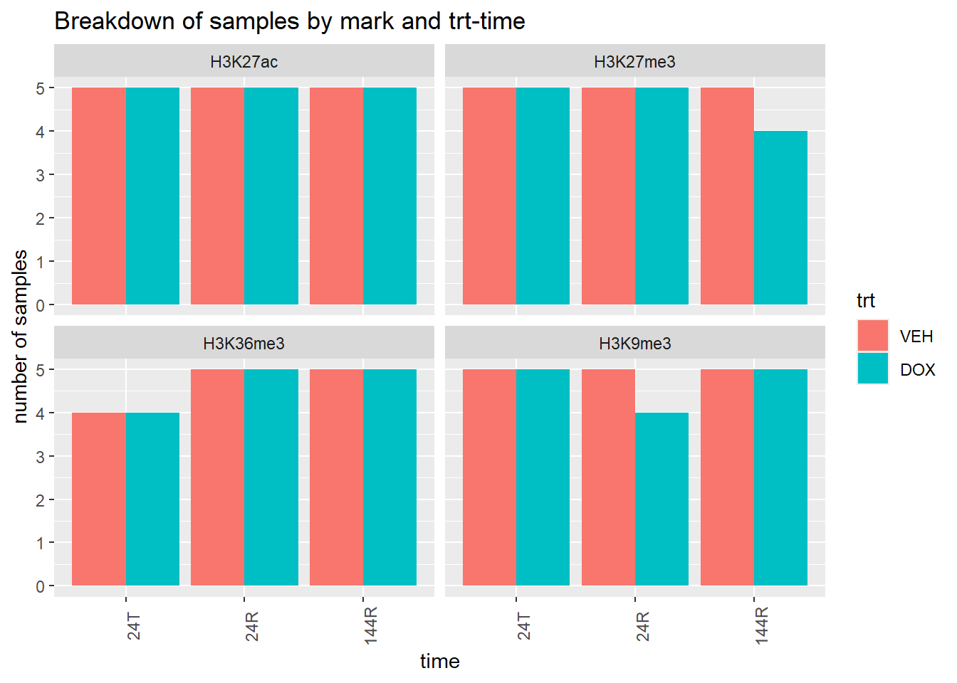
combo_trim_df %>%
  dplyr::filter(read=="R1") %>%
  group_by(trt,time,Histone_Mark) %>%
  tally() %>%
  pivot_wider(., id_cols=c(trt,time), names_from = Histone_Mark, values_from = n) %>%
  kable(.,caption = ("Sample counts")) %>%
  kable_paper("striped", full_width = FALSE) %>%
  kable_styling(full_width = FALSE,font_size = 16) %>%
scroll_box(width = "100%", height = "500px")| trt | time | H3K27ac | H3K27me3 | H3K36me3 | H3K9me3 |
|---|---|---|---|---|---|
| VEH | 24T | 5 | 5 | 4 | 5 |
| VEH | 24R | 5 | 5 | 5 | 5 |
| VEH | 144R | 5 | 5 | 5 | 5 |
| DOX | 24T | 5 | 5 | 4 | 5 |
| DOX | 24R | 5 | 5 | 5 | 4 |
| DOX | 144R | 5 | 4 | 5 | 5 |
Visualization of Counts
combo_trim_df %>%
  dplyr::filter(read=="R1") %>%
  ggplot(., aes(x = Sample, y= `Total Sequences`))+
  geom_col(aes(fill=Histone_Mark)) +
  theme(axis.text.x=element_text(vjust = .2,angle=90))+
  ylab("sequene count")+
  ggtitle("Paired End reads by sample and histone mark trimmed adapters")+
  scale_y_continuous( expand = expansion(mult = c(0, .1)))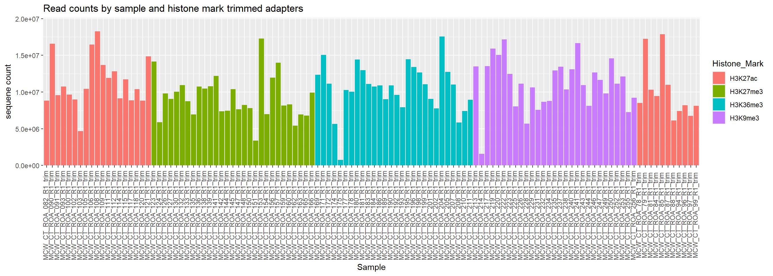
Tagging Questionable Libraries by Counts
questionable_ct <- combo_trim_df %>%
  dplyr::filter(`Total Sequences` < 2e6) %>%
  dplyr::select(Sample, `Total Sequences`) %>% distinct()
questionable_ct
# A tibble: 4 × 2
Sample `Total Sequences`
<chr> <dbl>
1 MCW_CT_ROA_175_R1_trim 734837
2 MCW_CT_ROA_175_R2_trim 734837
3 MCW_CT_ROA_214_R1_trim 1569281
4 MCW_CT_ROA_214_R2_trim 1569281combo_trim_df %>%
dplyr::filter(read=="R1") %>%
ggplot(., aes(x = Histone_Mark, y= `Total Sequences`))+
geom_boxplot(aes(fill=Histone_Mark)) +
geom_point(aes(color=ind))+
facet_wrap(trt~time)+
ylab("count")+
theme(axis.text.x=element_text(vjust = .2,angle=90))+
ggtitle("Paired end read count by trt and time, trimmed adapter")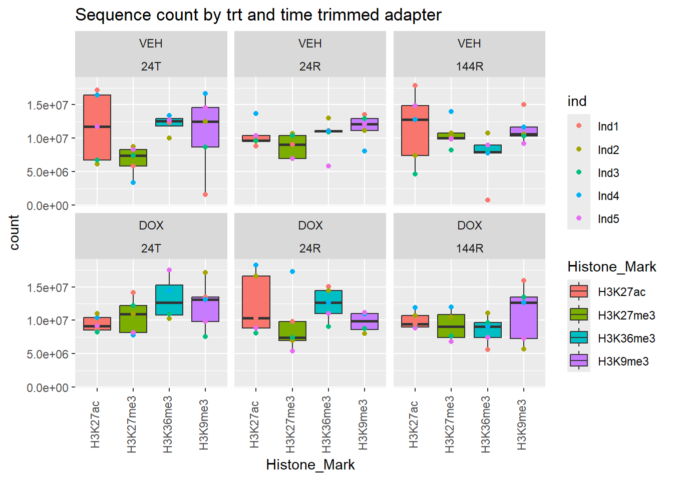
Trim Info
combo_trim_df %>%
  ggplot(., aes(x = read, y= avg_sequence_length))+
geom_boxplot(aes(fill=read))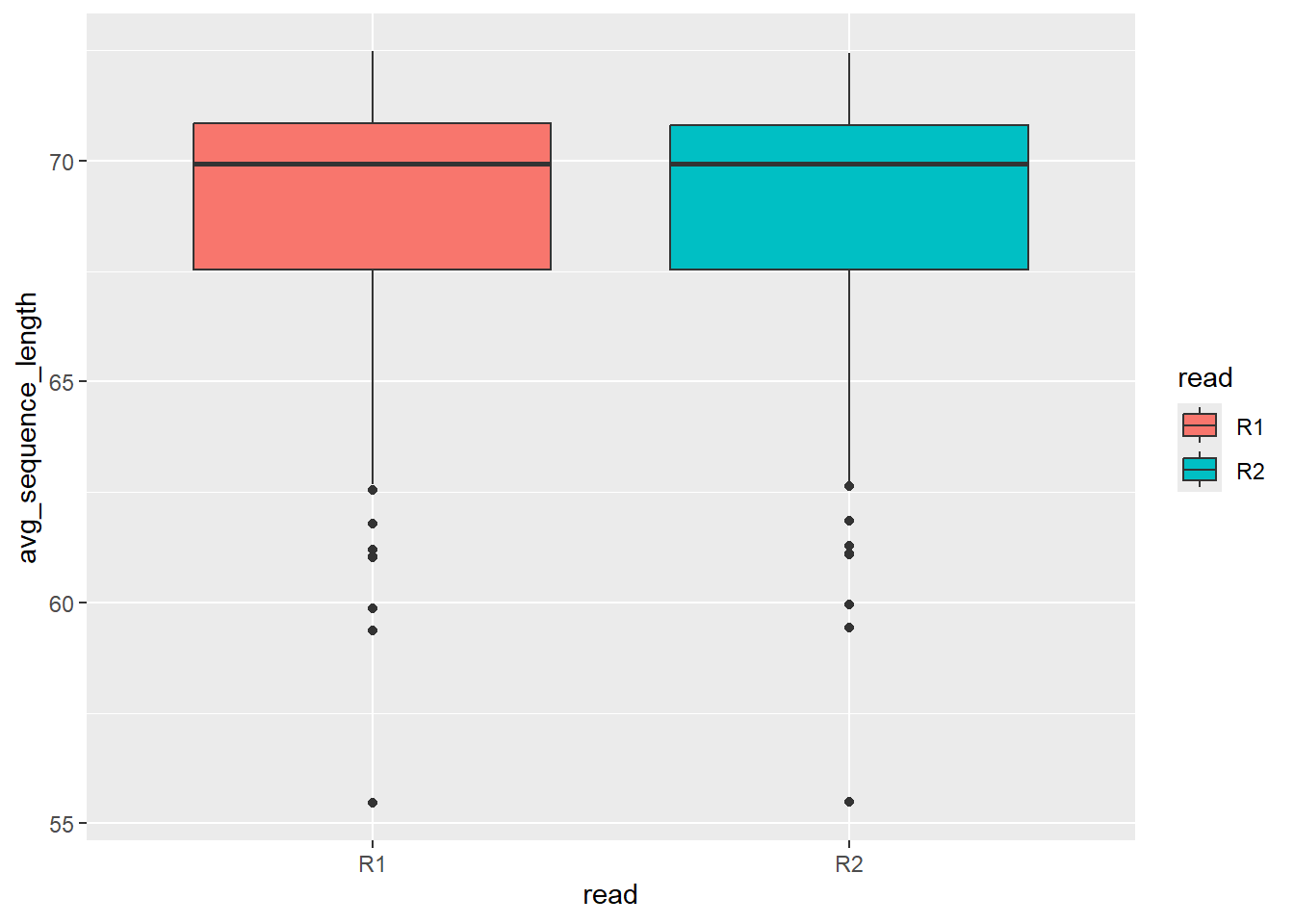
| Version | Author | Date |
|---|---|---|
| 0644589 | infurnoheat | 2025-07-02 |
combo_trim_df %>%
  ggplot(., aes(x = read, y= avg_sequence_length))+
geom_boxplot(aes(fill=Histone_Mark)) +
  ggtitle("Boxplot of trim read length across histone marks")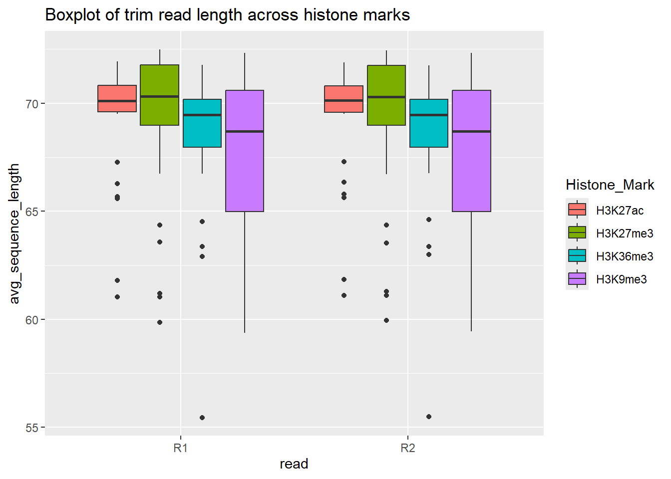
combo_trim_df %>%
  datatable(., options = list(scrollX = TRUE,
                              scrollY = "400px",
                              scrollCollapse = TRUE,
                              fixedColumns = list(leftColumns =2),
                              fixedHeader= TRUE),
            extensions = c("FixedColumns","Scroller"),
            class = "display")
# write_delim(combo_trim_df,"data/multiqc_data_trim/Summary_of_multiqcfiles.txt",delim = "\t")combo_trim_df %>%
dplyr::filter(read=="R1") %>%
ggplot(., aes(x = Sample, y= avg_sequence_length))+
geom_col(aes(fill=Histone_Mark)) +
geom_hline( yintercept = 75)+
theme_classic()+
ggtitle("Graph of average read length across R1 samples")+ theme(axis.text.x=element_text(vjust = .2,angle=90))+
scale_y_continuous( expand = expansion(mult = c(0, .1)))
combo_trim_df %>%
  dplyr::filter(read=="R2") %>%
  ggplot(., aes(x = Sample, y= avg_sequence_length))+
geom_col(aes(fill=Histone_Mark)) +
  geom_hline( yintercept = 75)+
  theme_classic()+
  ggtitle("Graph of average read length across R2 samples")+ theme(axis.text.x=element_text(vjust = .2,angle=90))+
  scale_y_continuous( expand = expansion(mult = c(0, .1)))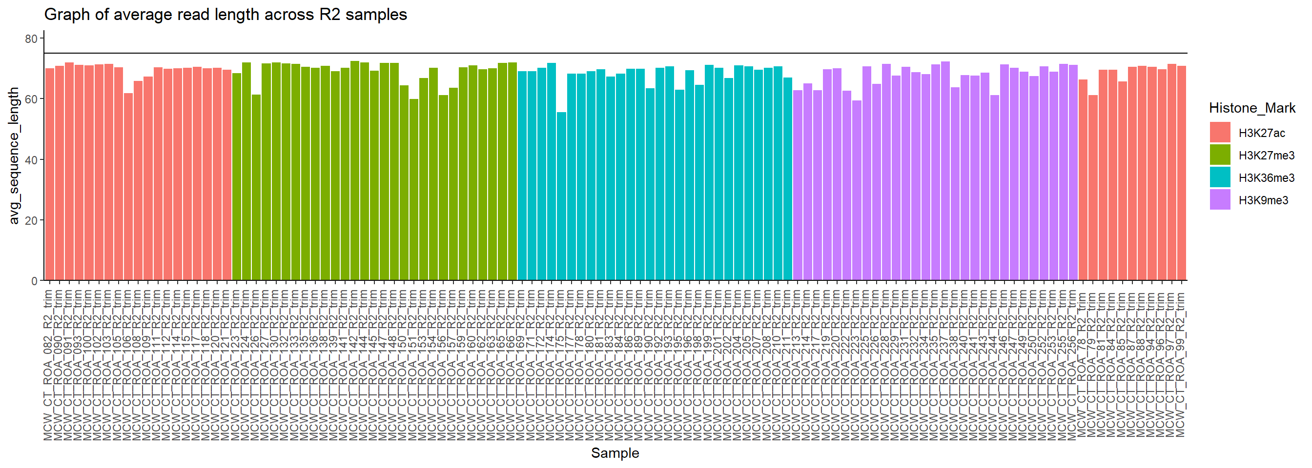
combo_trim_df %>%
  dplyr::filter(read=="R1") %>%
  ggplot(., aes(x = Sample, y= `%GC`))+
  geom_col(aes(fill=Histone_Mark)) +
  theme_classic()+
  ggtitle("Graph of %GC for R1 trimmed")+
  theme(axis.text.x=element_text(vjust = .2,angle=90))+
  scale_y_continuous( expand = expansion(mult = c(0, .1)))
combo_trim_df %>%
  dplyr::filter(read=="R2") %>%
  ggplot(., aes(x = Sample, y= `%GC`))+
  geom_col(aes(fill=Histone_Mark)) +
  theme_classic()+
  ggtitle("Graph of %GC for R2 trimmed")+
  theme(axis.text.x=element_text(vjust = .2,angle=90))+
  scale_y_continuous( expand = expansion(mult = c(0, .1)))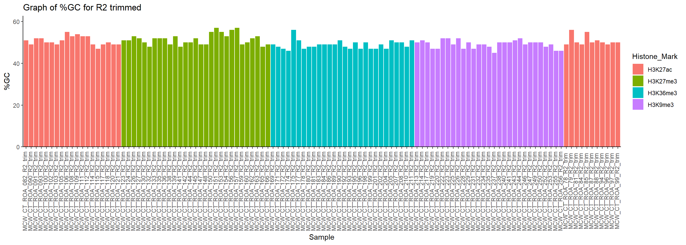
Duplication Info
combo_trim_df %>%
  dplyr::filter(read=="R1") %>%
  ggplot(., aes(x = Histone_Mark, y= `FastQC_mqc-generalstats-fastqc-percent_duplicates`))+
  geom_boxplot(aes(fill=Histone_Mark)) +
    geom_point(aes(color=ind))+
  facet_wrap(trt~time)+
  ylab("percent duplication")+
  theme(axis.text.x=element_text(angle=90))+
  ggtitle("Duplication percentage (R1 trimmed)")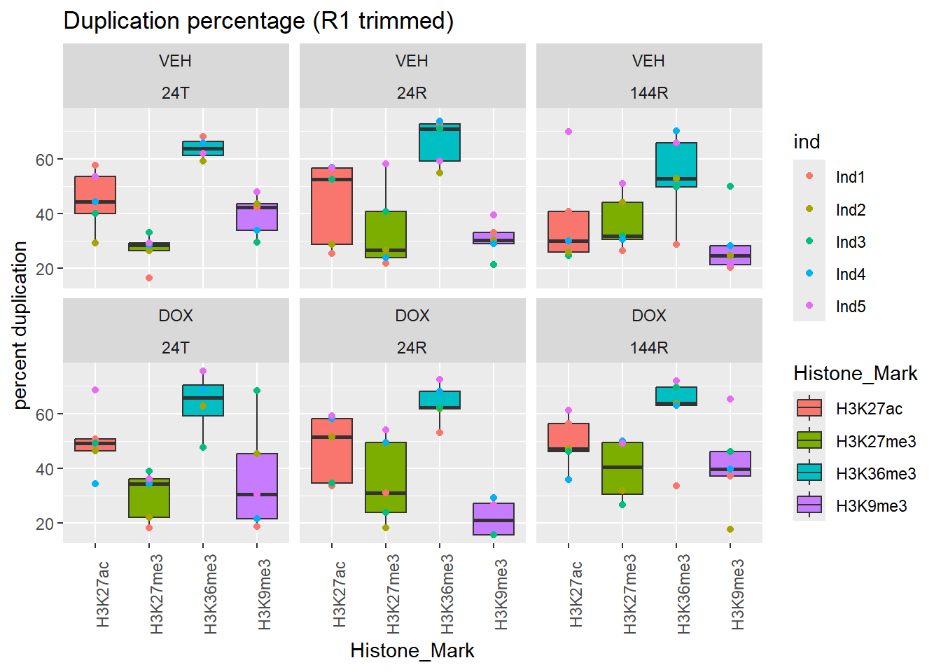
combo_trim_df %>%
  dplyr::filter(read=="R1") %>%
  ggplot(., aes(x = interaction(time,trt), y= `FastQC_mqc-generalstats-fastqc-percent_duplicates`))+
  geom_boxplot(aes(fill=Histone_Mark)) +
  geom_point(aes(color=ind))+
facet_wrap(~Histone_Mark)+
  ylab("percent duplication")+
  theme(axis.text.x=element_text(angle=90))+
  ggtitle("Duplication percentage (R1 trimmed)")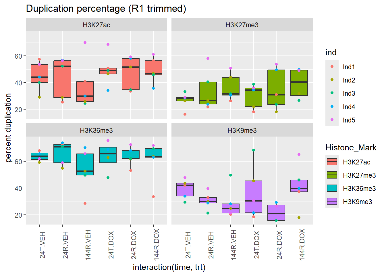
combo_trim_df %>%
  dplyr::filter(read=="R1") %>%
  ggplot(., aes(x = Sample, y= `FastQC_mqc-generalstats-fastqc-percent_duplicates`))+
  geom_col(aes(fill=Histone_Mark)) +
  theme_classic()+
  ggtitle("Graph of percent duplicates for R1 trimmed")+
  theme(axis.text.x=element_text(vjust = .2,angle=90))+
  scale_y_continuous( limits = c(0,100),expand = expansion(mult = c(0, .1)))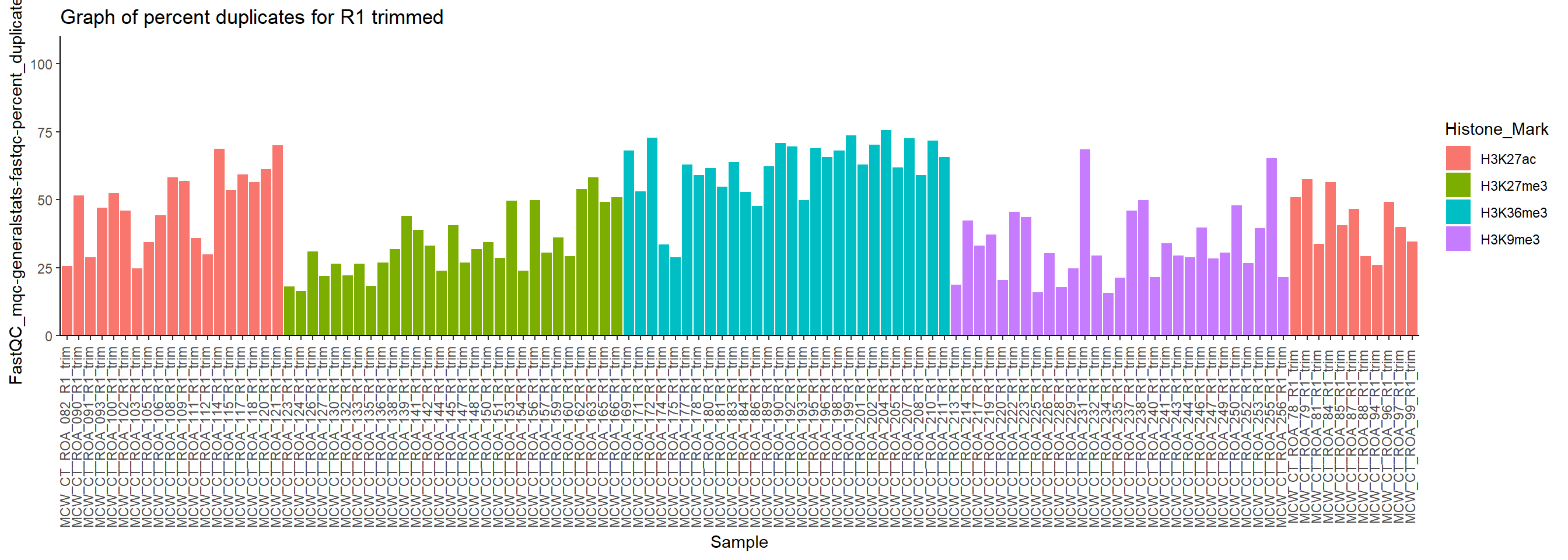
combo_trim_df %>%
  dplyr::filter(read=="R2") %>%
  ggplot(., aes(x = Sample, y= `FastQC_mqc-generalstats-fastqc-percent_duplicates`))+
  geom_col(aes(fill=Histone_Mark)) +
  theme_classic()+
  ggtitle("Graph of percent duplicates for R2 trimmed")+
  theme(axis.text.x=element_text(vjust = .2,angle=90))+
  scale_y_continuous(limits = c(0,100), expand = expansion(mult = c(0, .1)))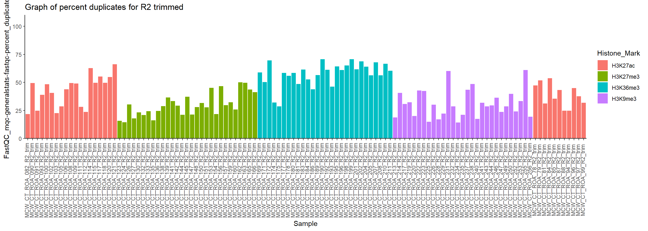
Alignment Analysis
Data Initialization
alignResult = c()
for(sample in sampleinfo$`Library ID`){
  alignRes = read.table(paste0("data/sams/", sample, ".log"), header = FALSE, fill = TRUE)
  alignRate = substr(alignRes$V1[6], 1, nchar(as.character(alignRes$V1[6]))-1)
  alignResult = data.frame(ID = sample,
                           Paired_Reads = alignRes$V1[1] %>% as.character %>% as.numeric,
                           aligned_concordant_0 = alignRes$V1[3] %>% as.character %>% as.numeric,
                           aligned_concordant_1 = alignRes$V1[4] %>% as.character %>% as.numeric,
                           aligned_concordant_g1 = alignRes$V1[5] %>% as.character %>% as.numeric,
                           MappedFragNum_hg38 = alignRes$V1[4] %>% as.character %>% as.numeric + alignRes$V1[5] %>% as.character %>% as.numeric,
                           percent_alignment = alignRate %>% as.numeric)  %>% rbind(alignResult, .)
}
alignResult %>% mutate(percent_alignment = paste0(percent_alignment, "%"))
ID Paired_Reads aligned_concordant_0 aligned_concordant_1
1 MCW_CT_ROA_78 8514537 393880 4454677
2 MCW_CT_ROA_79 17230410 750321 10921835
3 MCW_CT_ROA_80 11073255 513904 6094802
4 MCW_CT_ROA_81 10304161 342605 6909479
5 MCW_CT_ROA_082 8830034 388284 5998847
6 MCW_CT_ROA_83 13873472 496709 9607312
7 MCW_CT_ROA_84 9460829 320932 6281523
8 MCW_CT_ROA_85 17871310 609752 12887951
9 MCW_CT_ROA_86 7129722 264900 4998439
10 MCW_CT_ROA_87 10992015 398747 7180888
11 MCW_CT_ROA_88 6136901 231003 4367664
12 MCW_CT_ROA_89 10476954 351625 7372185
13 MCW_CT_ROA_090 16578704 608091 11417139
14 MCW_CT_ROA_091 9570470 354970 6845785
15 MCW_CT_ROA_093 10733977 519575 7639342
16 MCW_CT_ROA_94 7398484 206181 5202764
17 MCW_CT_ROA_95 9244604 533245 5462429
18 MCW_CT_ROA_96 8197575 503975 4828923
19 MCW_CT_ROA_97 6738747 290949 4109592
20 MCW_CT_ROA_99 8097526 351319 5337230
21 MCW_CT_ROA_100 9646404 486736 5746445
22 MCW_CT_ROA_101 5971251 172784 4279384
23 MCW_CT_ROA_102 8994528 397337 5895789
24 MCW_CT_ROA_103 4663599 213987 3024586
25 MCW_CT_ROA_105 10410306 643616 6984311
26 MCW_CT_ROA_106 16439638 740825 10332902
27 MCW_CT_ROA_107 14094464 546132 9669822
28 MCW_CT_ROA_108 18259872 1011915 11565498
29 MCW_CT_ROA_109 13689268 694161 8788342
30 MCW_CT_ROA_111 11910243 633389 7877522
31 MCW_CT_ROA_112 12803412 584653 9061482
32 MCW_CT_ROA_113 12211077 565919 7290370
33 MCW_CT_ROA_114 9122059 489242 5678494
34 MCW_CT_ROA_115 11702871 334002 7501717
35 MCW_CT_ROA_116 11303005 517995 6793739
36 MCW_CT_ROA_117 8839709 498148 5496942
37 MCW_CT_ROA_118 10368651 570077 5963755
38 MCW_CT_ROA_119 10678026 773463 5451719
39 MCW_CT_ROA_120 8814196 546081 5452486
40 MCW_CT_ROA_121 14847165 1629782 6092487
41 MCW_CT_ROA_167 10254437 534908 3892332
42 MCW_CT_ROA_169 12361299 382520 4997060
43 MCW_CT_ROA_171 15049027 361793 7562957
44 MCW_CT_ROA_172 11124138 325848 3611930
45 MCW_CT_ROA_173 12820367 319403 6889739
46 MCW_CT_ROA_174 5638348 131069 3468729
47 MCW_CT_ROA_175 734837 28434 371197
48 MCW_CT_ROA_177 10266750 391316 4669078
49 MCW_CT_ROA_178 10051149 469934 3751581
50 MCW_CT_ROA_180 14437895 365222 6234032
51 MCW_CT_ROA_181 12982038 310000 5865365
52 MCW_CT_ROA_183 11071957 326006 4366138
53 MCW_CT_ROA_184 10755984 277894 4608170
54 MCW_CT_ROA_185 10371500 329493 4739964
55 MCW_CT_ROA_186 10900502 240755 6123832
56 MCW_CT_ROA_189 9018945 281692 4431648
57 MCW_CT_ROA_190 10900566 385116 4348651
58 MCW_CT_ROA_192 9617315 299599 4183944
59 MCW_CT_ROA_193 7903839 177953 3799403
60 MCW_CT_ROA_194 13338827 346582 5058731
61 MCW_CT_ROA_195 14457362 533494 5876489
62 MCW_CT_ROA_196 13394379 616842 4576594
63 MCW_CT_ROA_198 12671191 571712 4766820
64 MCW_CT_ROA_199 11060140 262080 3187035
65 MCW_CT_ROA_201 9042663 267789 3320726
66 MCW_CT_ROA_202 7751943 236557 3106251
67 MCW_CT_ROA_204 17543011 1254631 7582032
68 MCW_CT_ROA_205 12747766 452055 6346330
69 MCW_CT_ROA_206 8455460 285711 4130128
70 MCW_CT_ROA_207 11006304 505492 5110713
71 MCW_CT_ROA_208 5856849 261315 2913687
72 MCW_CT_ROA_209 11297824 678861 4742105
73 MCW_CT_ROA_210 7400743 453340 3172790
74 MCW_CT_ROA_211 8938017 498894 3921761
75 MCW_CT_ROA_123 14153840 285442 10129373
76 MCW_CT_ROA_124 5862953 113298 4569976
77 MCW_CT_ROA_125 13609246 307506 10291964
78 MCW_CT_ROA_126 9817049 228387 7061107
79 MCW_CT_ROA_127 9069762 210990 7035945
80 MCW_CT_ROA_130 10036729 144062 7735497
81 MCW_CT_ROA_132 10953823 143726 8416880
82 MCW_CT_ROA_133 8741438 178478 6688236
83 MCW_CT_ROA_135 6948539 181264 5196535
84 MCW_CT_ROA_136 10720711 254421 7991394
85 MCW_CT_ROA_138 10446106 153712 7973512
86 MCW_CT_ROA_139 10762175 238762 8064720
87 MCW_CT_ROA_140 8720469 177782 6784325
88 MCW_CT_ROA_141 12193521 157429 9284343
89 MCW_CT_ROA_142 7383669 133449 5801304
90 MCW_CT_ROA_144 7436416 146205 5761043
91 MCW_CT_ROA_145 10381840 169224 7791123
92 MCW_CT_ROA_146 12450965 264074 9158338
93 MCW_CT_ROA_147 7627631 141979 5873262
94 MCW_CT_ROA_148 8242133 128801 6363806
95 MCW_CT_ROA_149 16699371 420261 12588934
96 MCW_CT_ROA_150 7813241 249723 5839994
97 MCW_CT_ROA_151 3381332 111822 2489439
98 MCW_CT_ROA_153 17281183 585576 12636036
99 MCW_CT_ROA_154 6988957 175769 5294346
100 MCW_CT_ROA_156 11950951 283389 8870887
101 MCW_CT_ROA_157 13986120 541326 10211147
102 MCW_CT_ROA_158 8616090 134093 6537637
103 MCW_CT_ROA_159 8134850 113982 6121793
104 MCW_CT_ROA_160 8326979 170965 6240943
105 MCW_CT_ROA_162 5424324 134268 4090158
106 MCW_CT_ROA_163 6954866 184684 5222610
107 MCW_CT_ROA_165 6796188 180535 5210420
108 MCW_CT_ROA_166 9900924 239075 7571148
109 MCW_CT_ROA_213 13499581 257693 7311755
110 MCW_CT_ROA_214 1569281 109424 688084
111 MCW_CT_ROA_215 12237851 278718 5844416
112 MCW_CT_ROA_217 13521248 334225 6700522
113 MCW_CT_ROA_218 15777772 345599 8119847
114 MCW_CT_ROA_219 15900601 313322 8501928
115 MCW_CT_ROA_220 15061110 230197 8078127
116 MCW_CT_ROA_221 11674777 334843 5875284
117 MCW_CT_ROA_222 17147873 390356 9336829
118 MCW_CT_ROA_223 12465025 317913 6133660
119 MCW_CT_ROA_224 7822917 196131 3787480
120 MCW_CT_ROA_225 8022702 184210 4517598
121 MCW_CT_ROA_226 11120375 348306 5648597
122 MCW_CT_ROA_227 11811856 259234 5996517
123 MCW_CT_ROA_228 5703944 109692 3137321
124 MCW_CT_ROA_229 10611034 244570 5424718
125 MCW_CT_ROA_230 8628302 163823 4562488
126 MCW_CT_ROA_231 7583015 512080 3953510
127 MCW_CT_ROA_232 8665986 227318 4543469
128 MCW_CT_ROA_233 11430178 234246 5907899
129 MCW_CT_ROA_234 8763664 178542 4688318
130 MCW_CT_ROA_235 12949588 202560 6967506
131 MCW_CT_ROA_236 9761129 170963 5457706
132 MCW_CT_ROA_237 13450470 220297 7381836
133 MCW_CT_ROA_238 10348384 337923 5139928
134 MCW_CT_ROA_239 11412974 275040 5757179
135 MCW_CT_ROA_240 13078783 360579 6821521
136 MCW_CT_ROA_241 16654461 410674 7543488
137 MCW_CT_ROA_243 10920806 277618 5557589
138 MCW_CT_ROA_244 8099611 293122 3505531
139 MCW_CT_ROA_245 10824038 357471 5000814
140 MCW_CT_ROA_246 12674448 307254 5903745
141 MCW_CT_ROA_247 11631878 281223 5176881
142 MCW_CT_ROA_249 9780958 294833 5647927
143 MCW_CT_ROA_250 14577232 447522 8040186
144 MCW_CT_ROA_252 11121551 227263 6209333
145 MCW_CT_ROA_253 12107678 374882 6464556
146 MCW_CT_ROA_254 7120797 355006 3843884
147 MCW_CT_ROA_255 7255699 557352 4441174
148 MCW_CT_ROA_256 9209722 205492 5168231
aligned_concordant_g1 MappedFragNum_hg38 percent_alignment
1 3665980 8120657 95.37%
2 5558254 16480089 95.65%
3 4464549 10559351 95.36%
4 3052077 9961556 96.68%
5 2442903 8441750 95.6%
6 3769451 13376763 96.42%
7 2858374 9139897 96.61%
8 4373607 17261558 96.59%
9 1866383 6864822 96.28%
10 3412380 10593268 96.37%
11 1538234 5905898 96.24%
12 2753144 10125329 96.64%
13 4553474 15970613 96.33%
14 2369715 9215500 96.29%
15 2575060 10214402 95.16%
16 1989539 7192303 97.21%
17 3248930 8711359 94.23%
18 2864677 7693600 93.85%
19 2338206 6447798 95.68%
20 2408977 7746207 95.66%
21 3413223 9159668 94.95%
22 1519083 5798467 97.11%
23 2701402 8597191 95.58%
24 1425026 4449612 95.41%
25 2782379 9766690 93.82%
26 5365911 15698813 95.49%
27 3878510 13548332 96.13%
28 5682459 17247957 94.46%
29 4206765 12995107 94.93%
30 3399332 11276854 94.68%
31 3157277 12218759 95.43%
32 4354788 11645158 95.37%
33 2954323 8632817 94.64%
34 3867152 11368869 97.15%
35 3991271 10785010 95.42%
36 2844619 8341561 94.36%
37 3834819 9798574 94.5%
38 4452844 9904563 92.76%
39 2815629 8268115 93.8%
40 7124896 13217383 89.02%
41 5827197 9719529 94.78%
42 6981719 11978779 96.91%
43 7124277 14687234 97.6%
44 7186360 10798290 97.07%
45 5611225 12500964 97.51%
46 2038550 5507279 97.68%
47 335206 706403 96.13%
48 5206356 9875434 96.19%
49 5829634 9581215 95.32%
50 7838641 14072673 97.47%
51 6806673 12672038 97.61%
52 6379813 10745951 97.06%
53 5869920 10478090 97.42%
54 5302043 10042007 96.82%
55 4535915 10659747 97.79%
56 4305605 8737253 96.88%
57 6166799 10515450 96.47%
58 5133772 9317716 96.88%
59 3926483 7725886 97.75%
60 7933514 12992245 97.4%
61 8047379 13923868 96.31%
62 8200943 12777537 95.39%
63 7332659 12099479 95.49%
64 7611025 10798060 97.63%
65 5454148 8774874 97.04%
66 4409135 7515386 96.95%
67 8706348 16288380 92.85%
68 5949381 12295711 96.45%
69 4039621 8169749 96.62%
70 5390099 10500812 95.41%
71 2681847 5595534 95.54%
72 5876858 10618963 93.99%
73 3774613 6947403 93.87%
74 4517362 8439123 94.42%
75 3739025 13868398 97.98%
76 1179679 5749655 98.07%
77 3009776 13301740 97.74%
78 2527555 9588662 97.67%
79 1822827 8858772 97.67%
80 2157170 9892667 98.56%
81 2393217 10810097 98.69%
82 1874724 8562960 97.96%
83 1570740 6767275 97.39%
84 2474896 10466290 97.63%
85 2318882 10292394 98.53%
86 2458693 10523413 97.78%
87 1758362 8542687 97.96%
88 2751749 12036092 98.71%
89 1448916 7250220 98.19%
90 1529168 7290211 98.03%
91 2421493 10212616 98.37%
92 3028553 12186891 97.88%
93 1612390 7485652 98.14%
94 1749526 8113332 98.44%
95 3690176 16279110 97.48%
96 1723524 7563518 96.8%
97 780071 3269510 96.69%
98 4059571 16695607 96.61%
99 1518842 6813188 97.49%
100 2796675 11667562 97.63%
101 3233647 13444794 96.13%
102 1944360 8481997 98.44%
103 1899075 8020868 98.6%
104 1915071 8156014 97.95%
105 1199898 5290056 97.52%
106 1547572 6770182 97.34%
107 1405233 6615653 97.34%
108 2090701 9661849 97.59%
109 5930133 13241888 98.09%
110 771773 1459857 93.03%
111 6114717 11959133 97.72%
112 6486501 13187023 97.53%
113 7312326 15432173 97.81%
114 7085351 15587279 98.03%
115 6752786 14830913 98.47%
116 5464650 11339934 97.13%
117 7420688 16757517 97.72%
118 6013452 12147112 97.45%
119 3839306 7626786 97.49%
120 3320894 7838492 97.7%
121 5123472 10772069 96.87%
122 5556105 11552622 97.81%
123 2456931 5594252 98.08%
124 4941746 10366464 97.7%
125 3901991 8464479 98.1%
126 3117425 7070935 93.25%
127 3895199 8438668 97.38%
128 5288033 11195932 97.95%
129 3896804 8585122 97.96%
130 5779522 12747028 98.44%
131 4132460 9590166 98.25%
132 5848337 13230173 98.36%
133 4870533 10010461 96.73%
134 5380755 11137934 97.59%
135 5896683 12718204 97.24%
136 8700299 16243787 97.53%
137 5085599 10643188 97.46%
138 4300958 7806489 96.38%
139 5465753 10466567 96.7%
140 6463449 12367194 97.58%
141 6173774 11350655 97.58%
142 3838198 9486125 96.99%
143 6089524 14129710 96.93%
144 4684955 10894288 97.96%
145 5268240 11732796 96.9%
146 2921907 6765791 95.01%
147 2257173 6698347 92.32%
148 3835999 9004230 97.77%for_plots <- alignResult %>%
left_join(.,sampleinfo, by=c("ID"="Library ID"))%>%
dplyr::select(ID:aligned_concordant_0,aligned_concordant_1, aligned_concordant_g1,percent_alignment, Histone_Mark, Individual, Treatment, Timepoint) %>%
distinct()
for_plots <- for_plots[(!for_plots$Treatment %in% "5FU"),]
# write_delim(for_plots,"data/alignment_summary.txt",delim= "\t")Read Visualization
for_plots %>%
  group_by(Histone_Mark) %>%
  ggplot(., aes(x=ID, y=Paired_Reads))+
    geom_col(aes(fill = Histone_Mark)) +
  theme_classic()+
  ggtitle("Graph of total paired reads")+
  theme(axis.text.x=element_text(vjust = .2,angle=90))+
  scale_y_continuous( expand = expansion(mult = c(0, .1)))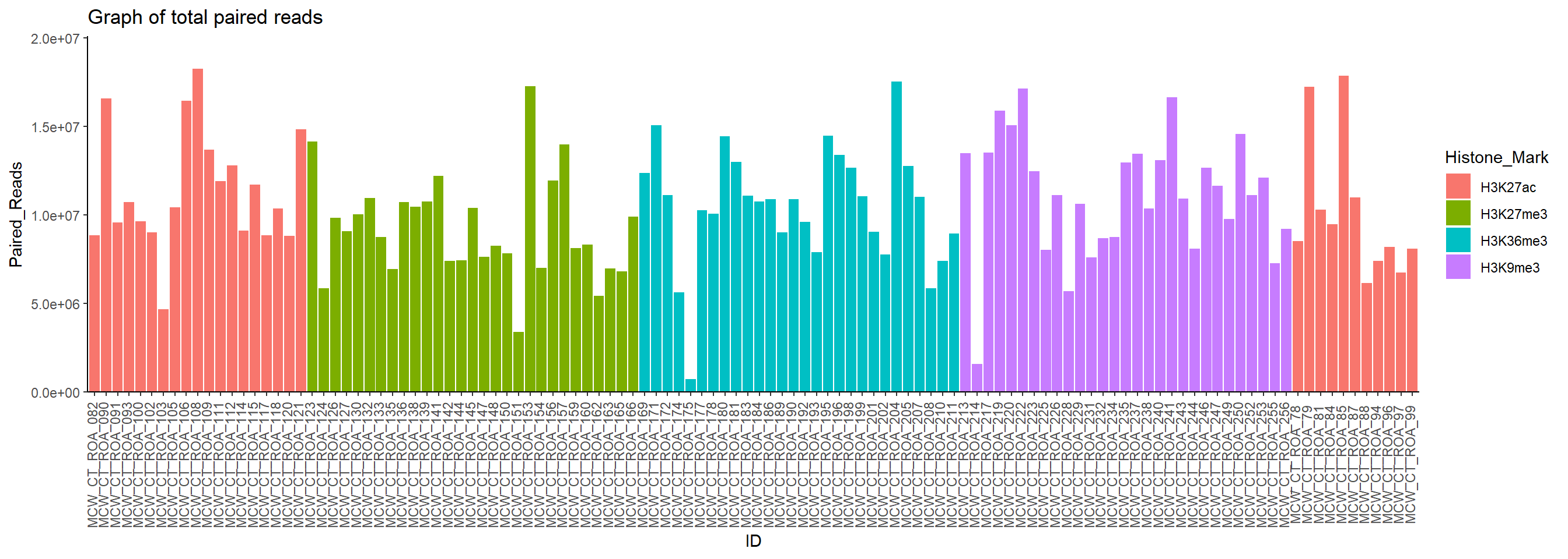
for_plots %>%
  group_by(Histone_Mark) %>%
  ggplot(., aes(x=ID, y=percent_alignment))+
    geom_col(aes(fill = Histone_Mark)) +
  theme_classic()+
  ggtitle("Percent aligned of paired reads") +
  theme(axis.text.x=element_text(vjust = .2,angle=90))+
  scale_y_continuous(expand = expansion(mult = c(0, .1)))+
  coord_cartesian(ylim=c(80,100))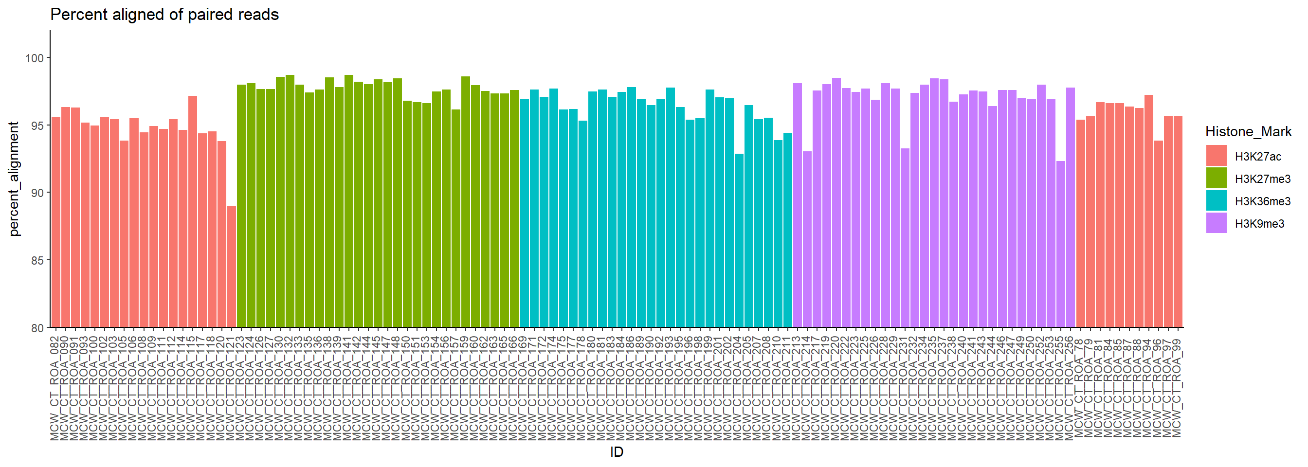
for_plots %>%
  group_by(Histone_Mark) %>%
   mutate(percent_aligned_unique = round(aligned_concordant_1 / Paired_Reads * 100, 2)) %>%
  ggplot(., aes(x=ID, y=percent_aligned_unique))+
    geom_col(aes(fill = Histone_Mark)) +
  theme_classic()+
  ggtitle("Percentage of paired reads aligning once")+
  theme(axis.text.x=element_text(vjust = .2,angle=90))+
  scale_y_continuous( expand = expansion(mult = c(0, .1)))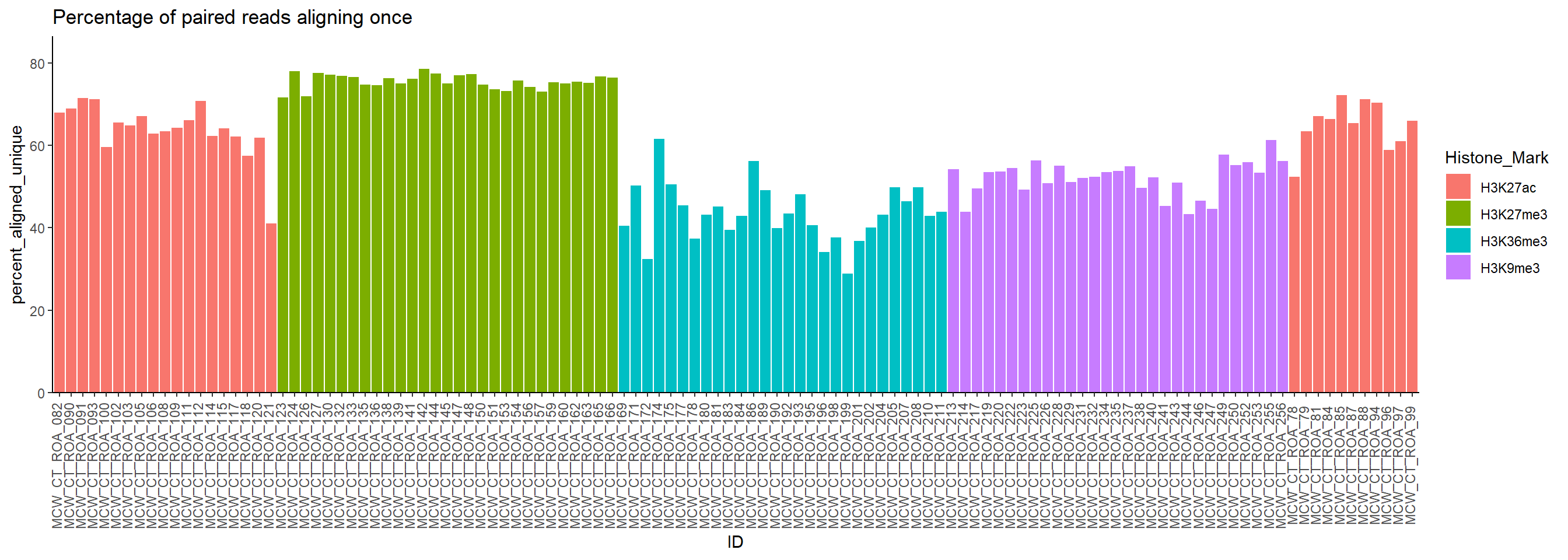
Read Analysis
Data Initialization
file_list_filter <- list.files(path="data/bam_no_multi",
           pattern ="frag_len_count\\.txt$",full.names = TRUE)
read_and_label <- function(file) {
  df <- read_delim(file, delim = "\t", col_names = c("Col1", "Col2"))  # Adjust delimiter if needed
  df <- df %>%
    mutate(File = basename(file),  # Add filename column
  weight = Col2/sum(Col2))
  return(df)
}
combined_df <- map_df(file_list_filter, read_and_label)

annotated_combo_df <- combined_df %>%
  mutate(sample = gsub("_frag_len_count.txt","",File)) %>%
  left_join(., sampleinfo, by = c("sample"="Library ID"))
annotated_combo_df <- annotated_combo_df[(!annotated_combo_df$Treatment %in% "5FU"),]
Read Visualization
annotated_combo_df %>%
  dplyr::filter(Histone_Mark=="H3K9me3") %>%
  ggplot(., aes(x=Col1, y=Col2, color = sample))+
  geom_line(size=1)+
  scale_x_continuous(breaks = seq(0, max(annotated_combo_df$Col1), by = 50))+
   facet_wrap(~sample)+
  labs(title = "Fragment length, H3K9me3",
       x = "Fragment Length (bp)",
       y = "Count",
       color= "Sample")+
  theme_minimal()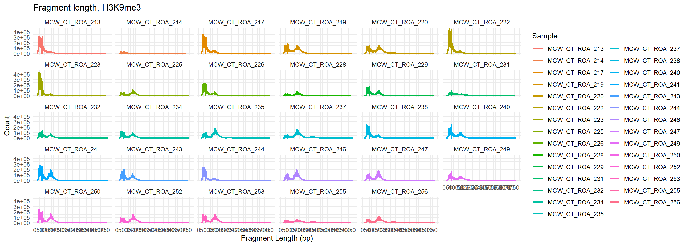
annotated_combo_df %>%
  dplyr::filter(Histone_Mark=="H3K9me3") %>%
  ggplot(., aes(x=sample, y=Col1, weight = weight,fill = Histone_Mark))+
geom_violin(bw = 5) +
    scale_y_continuous(breaks = seq(0, 800, 50)) +
   theme_bw(base_size = 20) +
    ggpubr::rotate_x_text(angle = 90) +
  ggtitle("Fragment lengths for H3K9me3")+
    ylab("Fragment Length") +
    xlab("")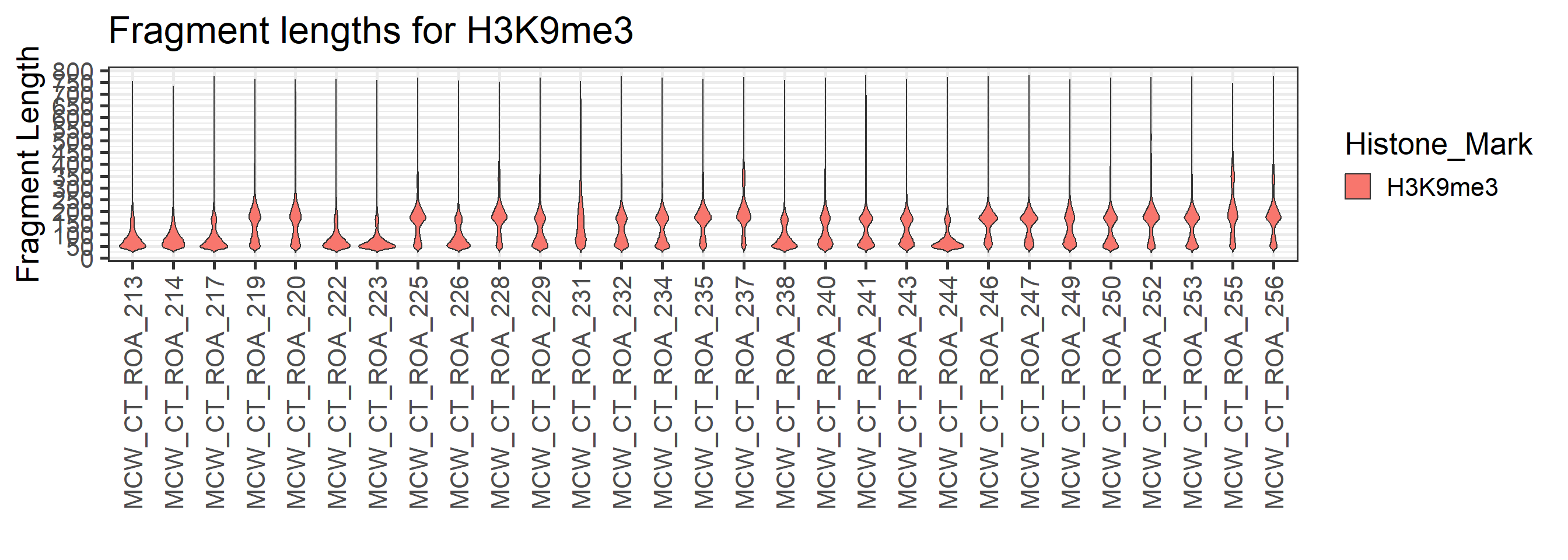
annotated_combo_df %>%
  dplyr::filter(Histone_Mark=="H3K27ac") %>%
  ggplot(., aes(x=Col1, y=Col2, color = sample))+
  geom_line(size=1)+
  scale_x_continuous(breaks = seq(0, max(annotated_combo_df$Col1), by = 50))+
   facet_wrap(~sample)+
  labs(title = "Fragment length, H3K27ac",
       x = "Fragment Length (bp)",
       y = "Count",
       color= "Sample")+
  theme_minimal()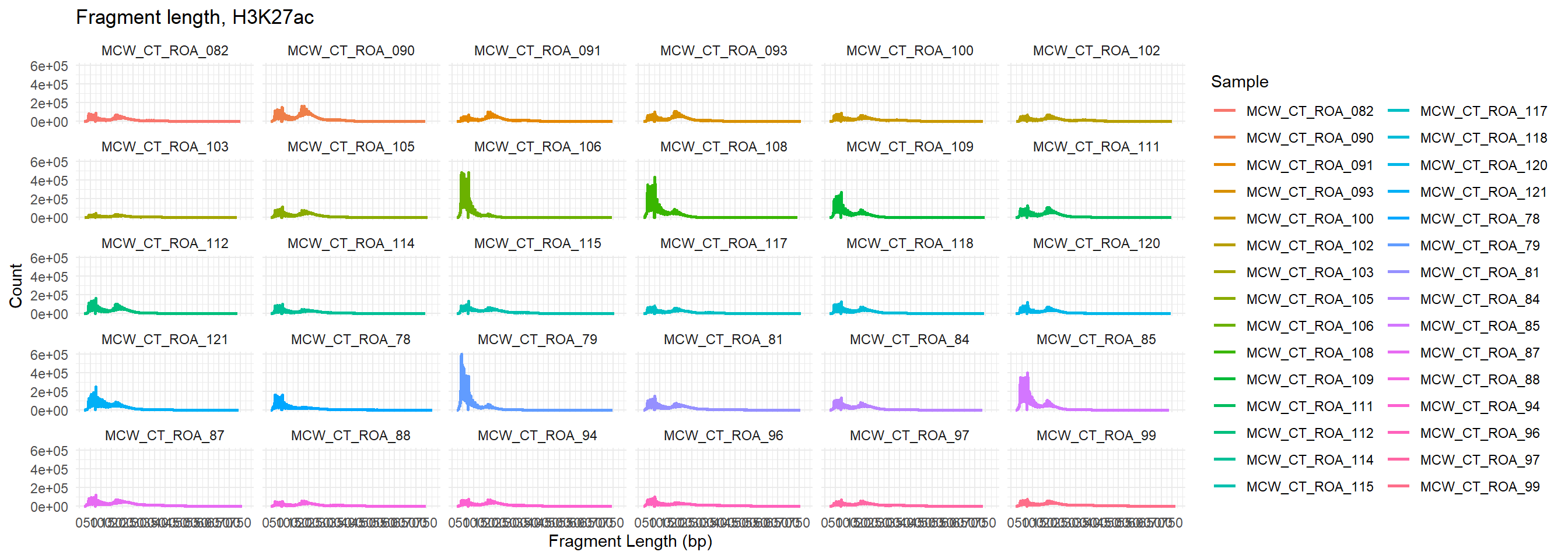
annotated_combo_df %>%
  dplyr::filter(Histone_Mark=="H3K27ac") %>%
  ggplot(., aes(x=sample, y=Col1, weight = weight,fill = Histone_Mark))+
geom_violin(bw = 5) +
    scale_y_continuous(breaks = seq(0, 800, 50)) +
   theme_bw(base_size = 20) +
    ggpubr::rotate_x_text(angle = 90) +
  ggtitle("Fragment lengths for H3K27ac")+
    ylab("Fragment Length") +
    xlab("")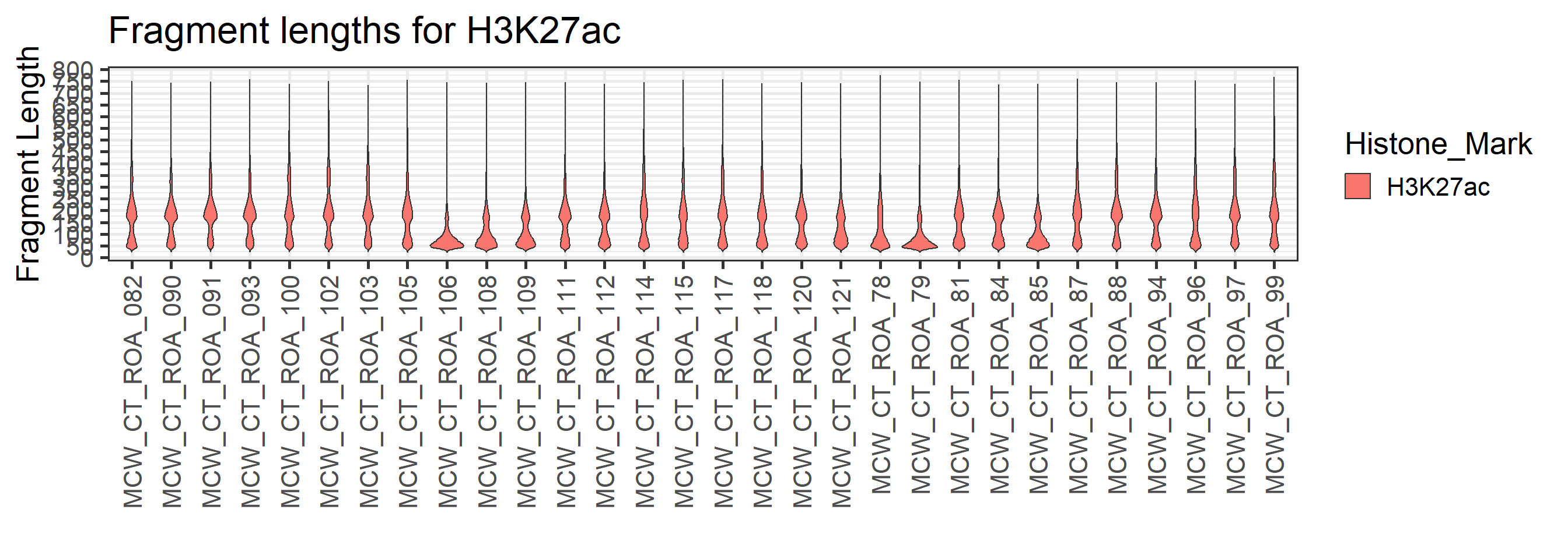
annotated_combo_df %>%
  dplyr::filter(Histone_Mark=="H3K27me3") %>%
  ggplot(., aes(x=Col1, y=Col2, color = sample))+
  geom_line(size=1)+
  scale_x_continuous(breaks = seq(0, max(annotated_combo_df$Col1), by = 50))+
   facet_wrap(~sample)+
  labs(title = "Fragment length, H3K27me3",
       x = "Fragment Length (bp)",
       y = "Count",
       color= "Sample")+
  theme_minimal()
annotated_combo_df %>%
  dplyr::filter(Histone_Mark=="H3K27me3") %>%
  ggplot(., aes(x=sample, y=Col1, weight = weight,fill = Histone_Mark))+
geom_violin(bw = 5) +
    scale_y_continuous(breaks = seq(0, 800, 50)) +
   theme_bw(base_size = 20) +
    ggpubr::rotate_x_text(angle = 90) +
  ggtitle("Fragment lengths for H3K27me3")+
    ylab("Fragment Length") +
    xlab("")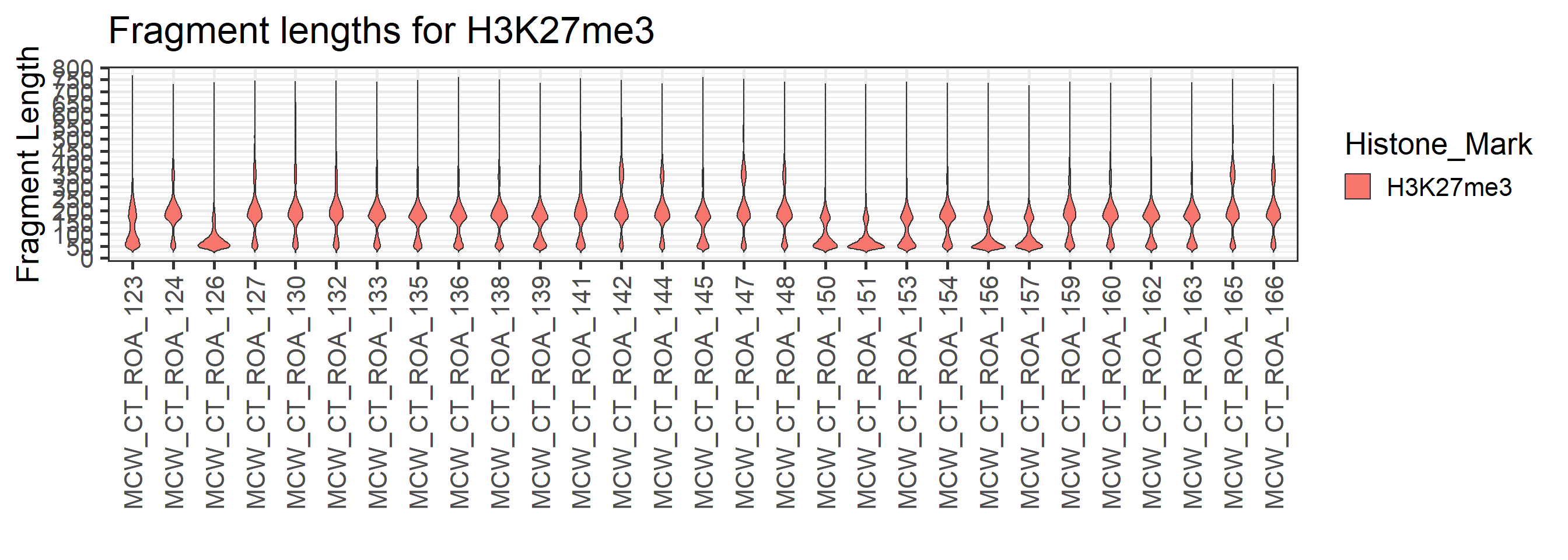
annotated_combo_df %>%
  dplyr::filter(Histone_Mark=="H3K36me3") %>%
  ggplot(., aes(x=Col1, y=Col2, color = sample))+
  geom_line(size=1)+
  scale_x_continuous(breaks = seq(0, max(annotated_combo_df$Col1), by = 50))+
   facet_wrap(~sample)+
  labs(title = "Fragment length, H3K36me3",
       x = "Fragment Length (bp)",
       y = "Count",
       color= "Sample")+
  theme_minimal()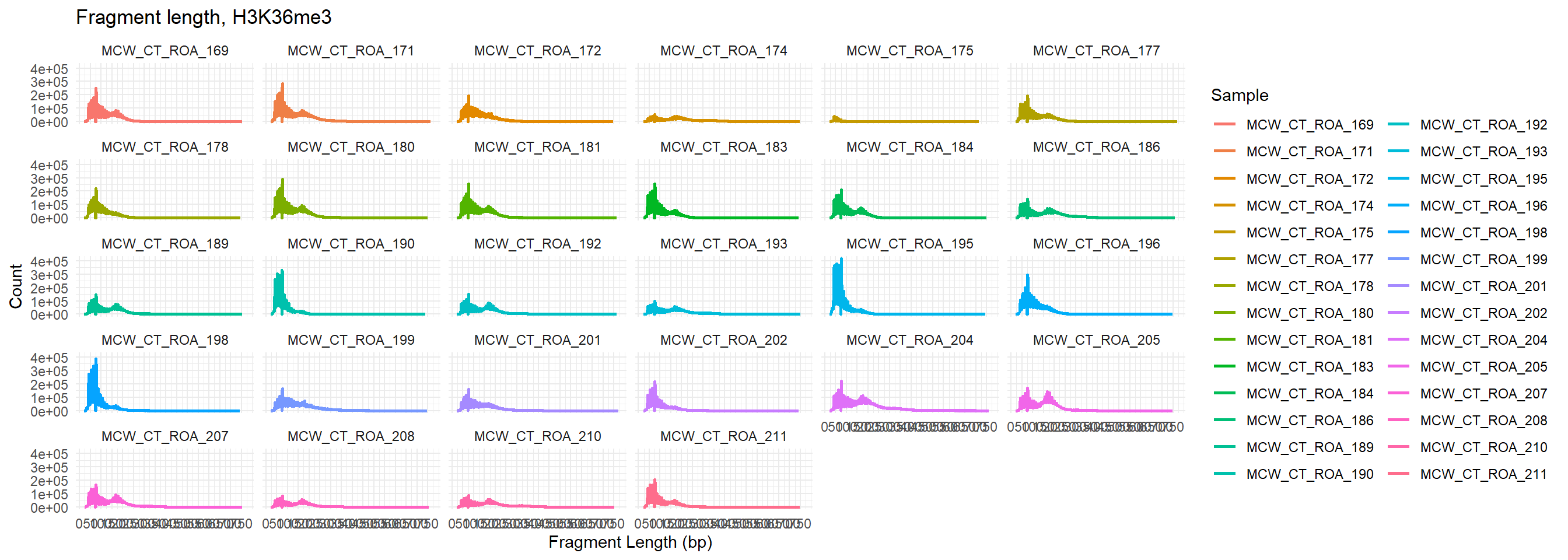
annotated_combo_df %>%
  dplyr::filter(Histone_Mark=="H3K36me3") %>%
  ggplot(., aes(x=sample, y=Col1, weight = weight,fill = Histone_Mark))+
geom_violin(bw = 5) +
    scale_y_continuous(breaks = seq(0, 800, 50)) +
   theme_bw(base_size = 20) +
    ggpubr::rotate_x_text(angle = 90) +
  ggtitle("Fragment lengths for H3K36me3")+
    ylab("Fragment Length") +
    xlab("")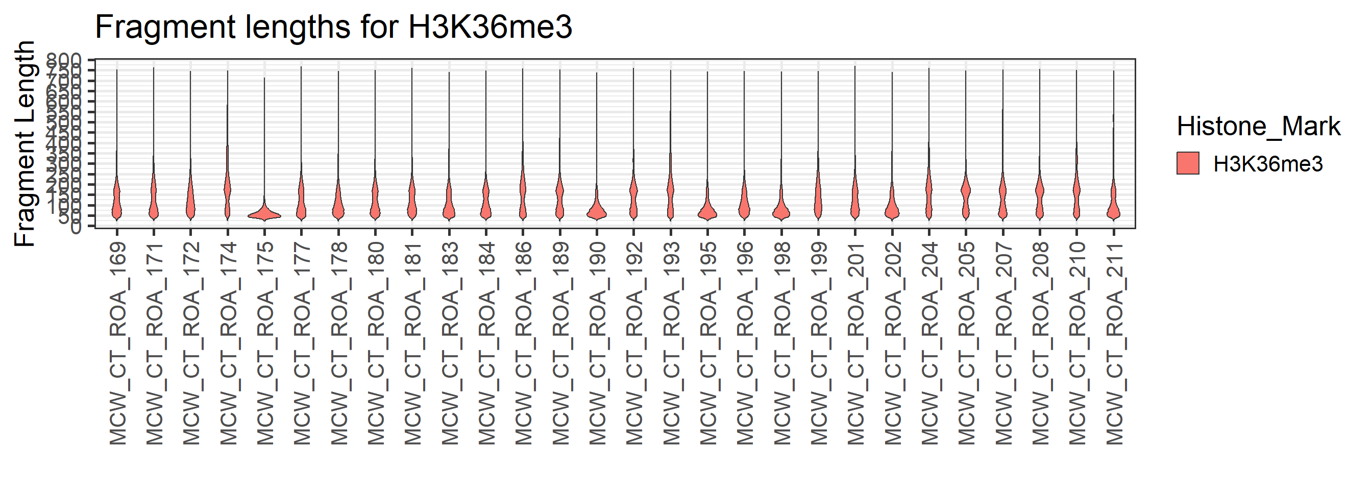
Tagging Questionable Libraries by Frag Len
peaks <- data.frame(sample = unique(annotated_combo_df$sample))
peaks[,"peakNum"] <- NA
for (s in peaks$sample) {
  weights <- annotated_combo_df %>%
    dplyr::filter(sample==s) %>%
    dplyr::select(Col1, weight)
  weights$smooth <- smooth_data(x = weights$Col1, y = weights$weight, sm_method = "moving-average", window_width_n = 15)
  weights$peak <- find_peaks(weights$smooth, span = 31, global.threshold = 0.01)
  peaks[peaks$sample == s,"peakNum"] <- sum(as.numeric(weights$peak[-1:-150]))
}
questionable_frag = peaks[(peaks$peakNum == 0),]
questionable_frag %>%
  left_join(., sampleinfo, by =c("sample"="Library ID"))
sample peakNum Histone_Mark Individual Treatment Timepoint
1 MCW_CT_ROA_126 0 H3K27me3 Ind1 DOX 24R
2 MCW_CT_ROA_151 0 H3K27me3 Ind4 VEH 24T
3 MCW_CT_ROA_169 0 H3K36me3 Ind1 VEH 24T
4 MCW_CT_ROA_172 0 H3K36me3 Ind1 VEH 24R
5 MCW_CT_ROA_175 0 H3K36me3 Ind1 VEH 144R
6 MCW_CT_ROA_178 0 H3K36me3 Ind2 VEH 24T
7 MCW_CT_ROA_181 0 H3K36me3 Ind2 VEH 24R
8 MCW_CT_ROA_183 0 H3K36me3 Ind2 DOX 144R
9 MCW_CT_ROA_190 0 H3K36me3 Ind3 VEH 24R
10 MCW_CT_ROA_195 0 H3K36me3 Ind4 DOX 24T
11 MCW_CT_ROA_196 0 H3K36me3 Ind4 VEH 24T
12 MCW_CT_ROA_198 0 H3K36me3 Ind4 DOX 24R
13 MCW_CT_ROA_201 0 H3K36me3 Ind4 DOX 144R
14 MCW_CT_ROA_202 0 H3K36me3 Ind4 VEH 144R
15 MCW_CT_ROA_211 0 H3K36me3 Ind5 VEH 144R
16 MCW_CT_ROA_213 0 H3K9me3 Ind1 DOX 24T
17 MCW_CT_ROA_214 0 H3K9me3 Ind1 VEH 24T
18 MCW_CT_ROA_217 0 H3K9me3 Ind1 VEH 24R
19 MCW_CT_ROA_222 0 H3K9me3 Ind2 DOX 24T
20 MCW_CT_ROA_223 0 H3K9me3 Ind2 VEH 24T
21 MCW_CT_ROA_226 0 H3K9me3 Ind2 VEH 24R
22 MCW_CT_ROA_238 0 H3K9me3 Ind3 VEH 144R
23 MCW_CT_ROA_241 0 H3K9me3 Ind4 VEH 24T
24 MCW_CT_ROA_244 0 H3K9me3 Ind4 VEH 24RRead Analysisafter Filtering
Data Initialization
file_list_noM <- list.files(path="data/bam_final",
           pattern ="frag_len_noM\\.txt$",full.names = TRUE)
read_and_label <- function(file) {
  df <- read_delim(file, delim = "\t", col_names = c("Col1", "Col2"))  # Adjust delimiter if needed
  df <- df %>%
    mutate(File = basename(file),  # Add filename column
  weight = Col2/sum(Col2))
  return(df)
}
combined_df <- map_df(file_list_noM, read_and_label)

annotated_noM_df <- combined_df %>%
  mutate(sample = gsub("_frag_len_noM.txt","",File)) %>%
  left_join(., sampleinfo, by = c("sample"="Library ID"))
annotated_noM_df <- annotated_noM_df[(!annotated_noM_df$Treatment %in% "5FU"),]
Read Visualization
annotated_noM_df %>%
  dplyr::filter(Histone_Mark=="H3K9me3") %>%
  ggplot(., aes(x=Col1, y=Col2, color = sample))+
  geom_line(size=1)+
  scale_x_continuous(breaks = seq(0, max(annotated_combo_df$Col1), by = 50))+
   facet_wrap(~sample)+
  labs(title = "Fragment length, H3K9me3",
       x = "Fragment Length (bp)",
       y = "Count",
       color= "Sample")+
  theme_minimal()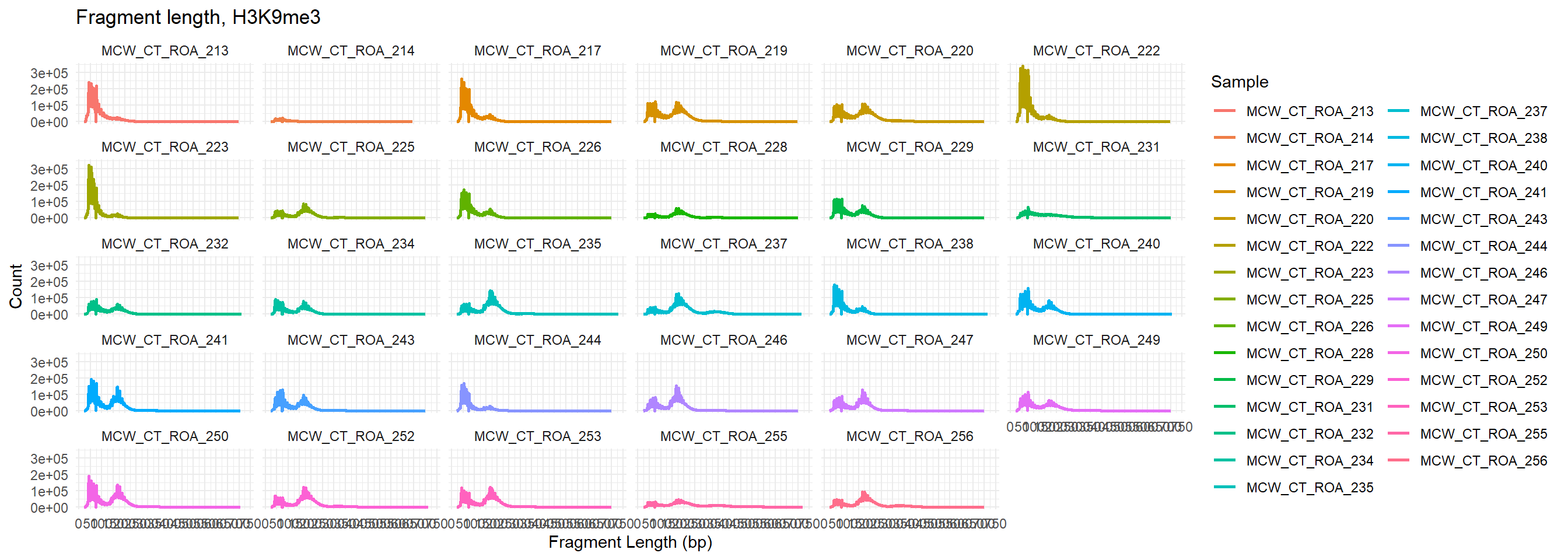
annotated_noM_df %>%
  dplyr::filter(Histone_Mark=="H3K9me3") %>%
  ggplot(., aes(x=sample, y=Col1, weight = weight,fill = Histone_Mark))+
geom_violin(bw = 5) +
    scale_y_continuous(breaks = seq(0, 800, 50)) +
   theme_bw(base_size = 20) +
    ggpubr::rotate_x_text(angle = 90) +
  ggtitle("Fragment lengths for H3K9me3")+
    ylab("Fragment Length") +
    xlab("")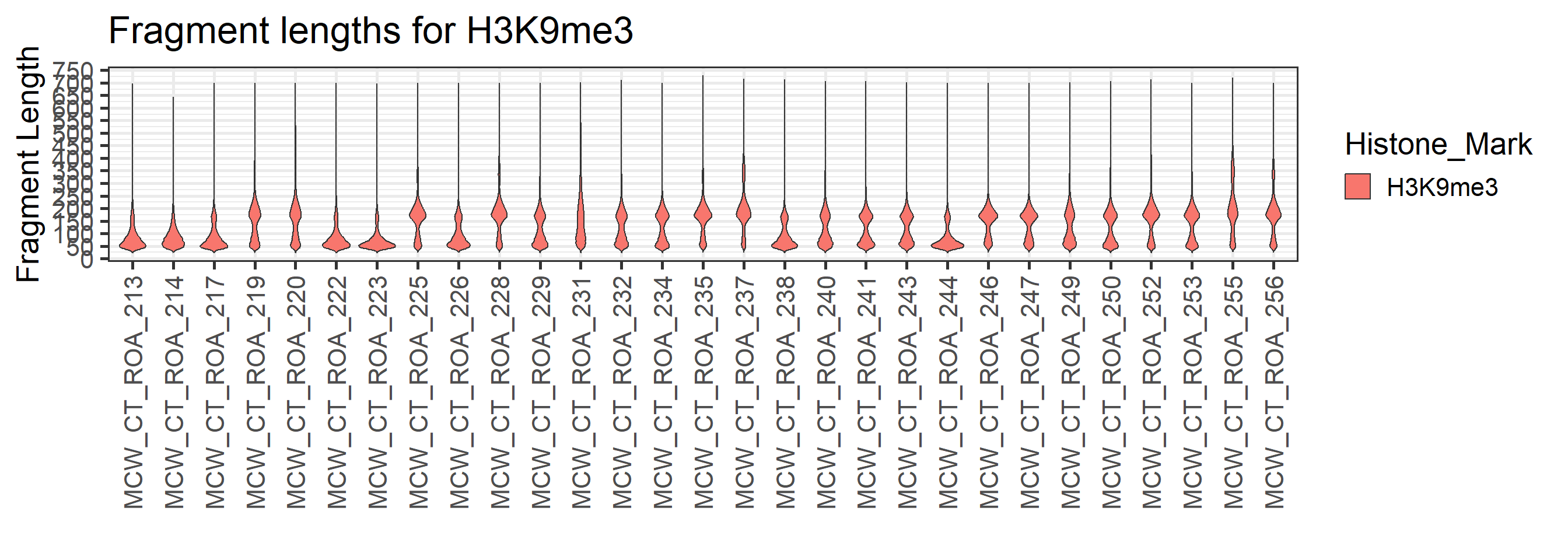
annotated_noM_df %>%
  dplyr::filter(Histone_Mark=="H3K27ac") %>%
  ggplot(., aes(x=Col1, y=Col2, color = sample))+
  geom_line(size=1)+
  scale_x_continuous(breaks = seq(0, max(annotated_combo_df$Col1), by = 50))+
   facet_wrap(~sample)+
  labs(title = "Fragment length, H3K27ac",
       x = "Fragment Length (bp)",
       y = "Count",
       color= "Sample")+
  theme_minimal()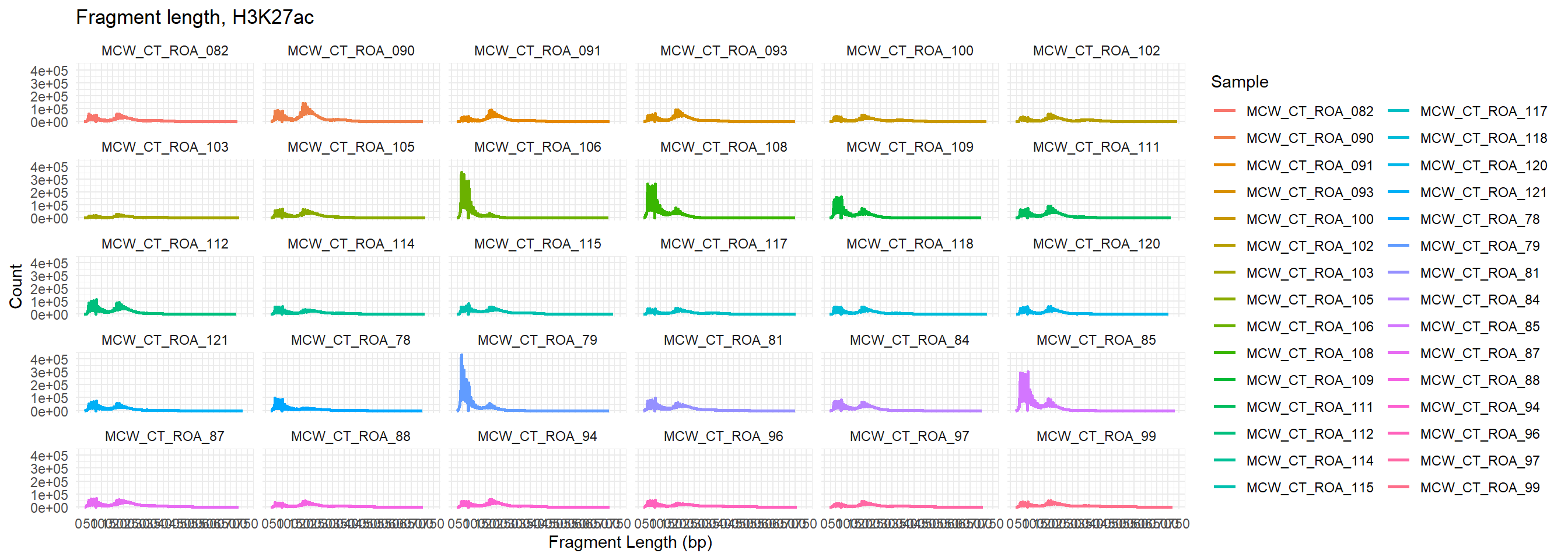
annotated_noM_df %>%
  dplyr::filter(Histone_Mark=="H3K27ac") %>%
  ggplot(., aes(x=sample, y=Col1, weight = weight,fill = Histone_Mark))+
geom_violin(bw = 5) +
    scale_y_continuous(breaks = seq(0, 800, 50)) +
   theme_bw(base_size = 20) +
    ggpubr::rotate_x_text(angle = 90) +
  ggtitle("Fragment lengths for H3K27ac")+
    ylab("Fragment Length") +
    xlab("")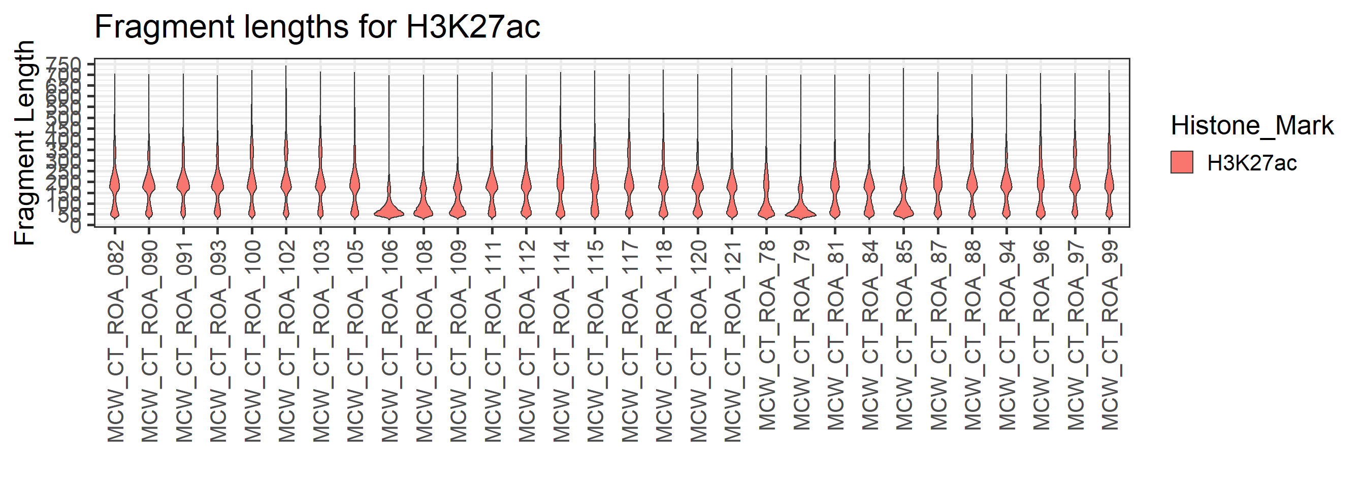
annotated_noM_df %>%
  dplyr::filter(Histone_Mark=="H3K27me3") %>%
  ggplot(., aes(x=Col1, y=Col2, color = sample))+
  geom_line(size=1)+
  scale_x_continuous(breaks = seq(0, max(annotated_combo_df$Col1), by = 50))+
   facet_wrap(~sample)+
  labs(title = "Fragment length, H3K27me3",
       x = "Fragment Length (bp)",
       y = "Count",
       color= "Sample")+
  theme_minimal()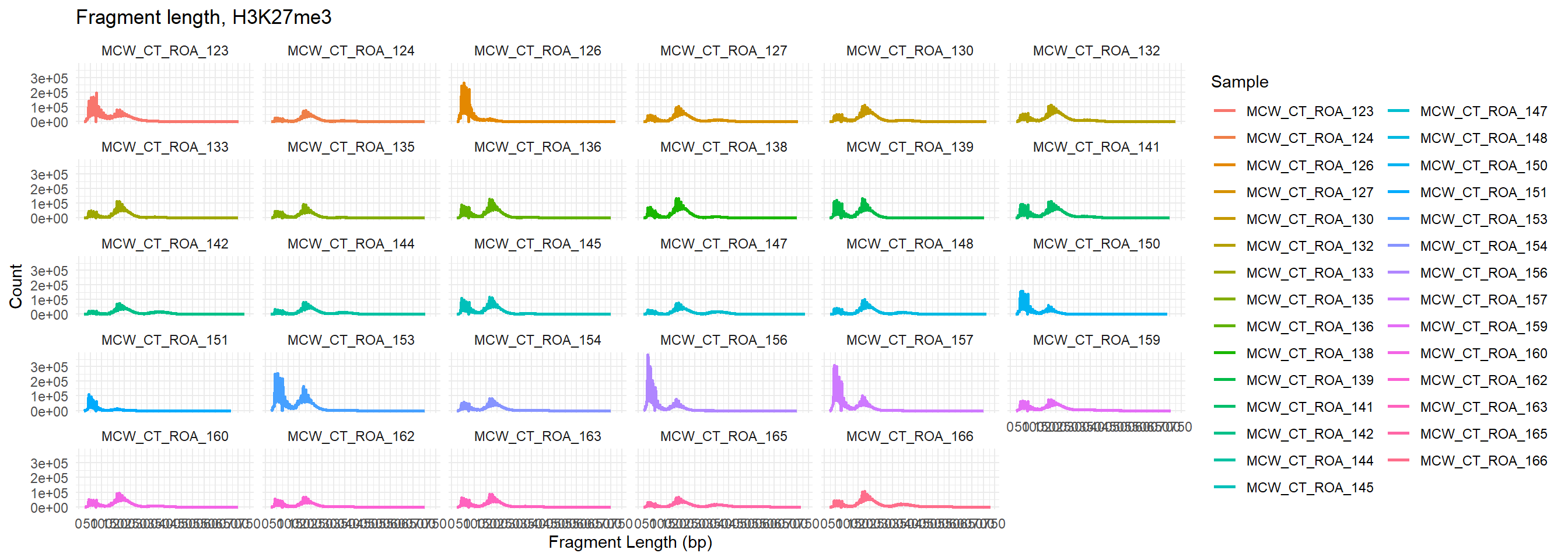
annotated_noM_df %>%
  dplyr::filter(Histone_Mark=="H3K27me3") %>%
  ggplot(., aes(x=sample, y=Col1, weight = weight,fill = Histone_Mark))+
geom_violin(bw = 5) +
    scale_y_continuous(breaks = seq(0, 800, 50)) +
   theme_bw(base_size = 20) +
    ggpubr::rotate_x_text(angle = 90) +
  ggtitle("Fragment lengths for H3K27me3")+
    ylab("Fragment Length") +
    xlab("")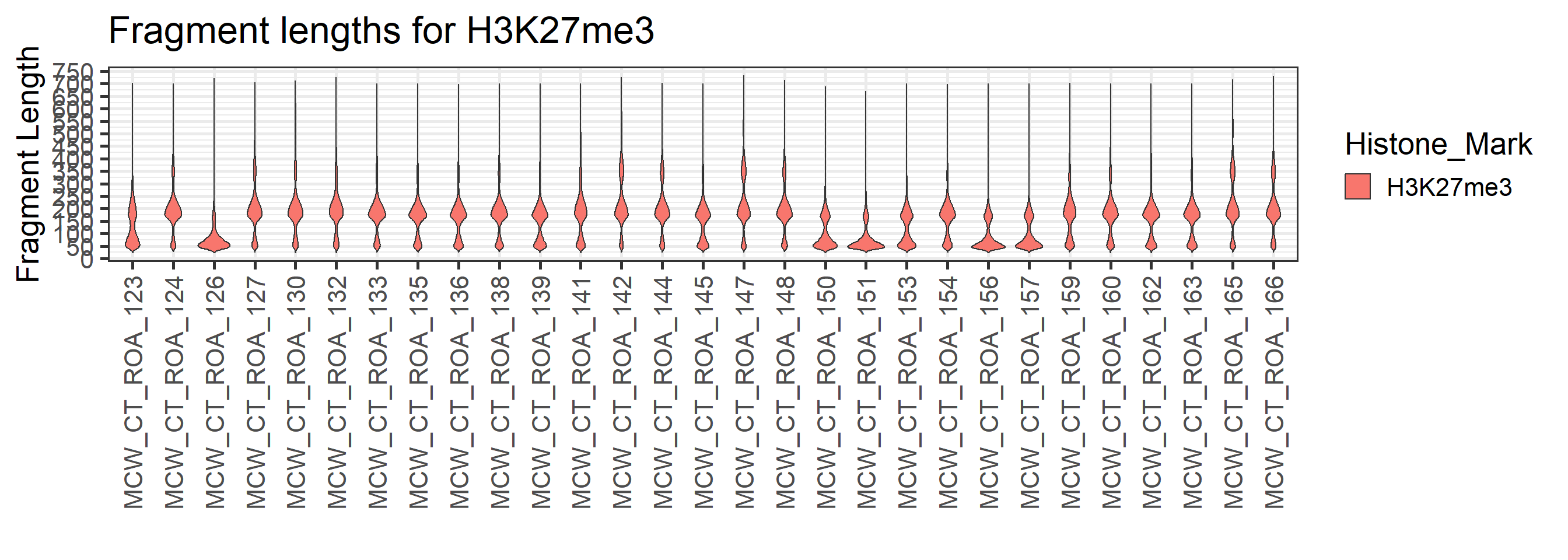
annotated_noM_df %>%
  dplyr::filter(Histone_Mark=="H3K36me3") %>%
  ggplot(., aes(x=Col1, y=Col2, color = sample))+
  geom_line(size=1)+
  scale_x_continuous(breaks = seq(0, max(annotated_combo_df$Col1), by = 50))+
   facet_wrap(~sample)+
  labs(title = "Fragment length, H3K36me3",
       x = "Fragment Length (bp)",
       y = "Count",
       color= "Sample")+
  theme_minimal()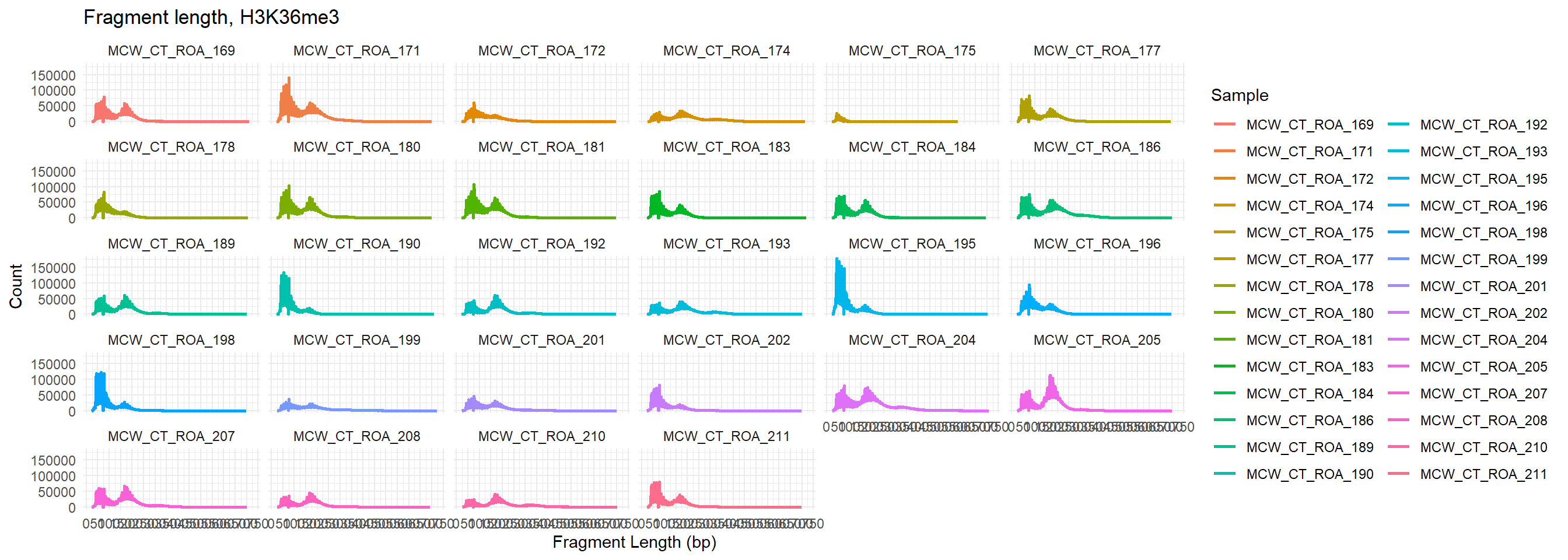
annotated_noM_df %>%
  dplyr::filter(Histone_Mark=="H3K36me3") %>%
  ggplot(., aes(x=sample, y=Col1, weight = weight,fill = Histone_Mark))+
geom_violin(bw = 5) +
    scale_y_continuous(breaks = seq(0, 800, 50)) +
   theme_bw(base_size = 20) +
    ggpubr::rotate_x_text(angle = 90) +
  ggtitle("Fragment lengths for H3K36me3")+
    ylab("Fragment Length") +
    xlab("")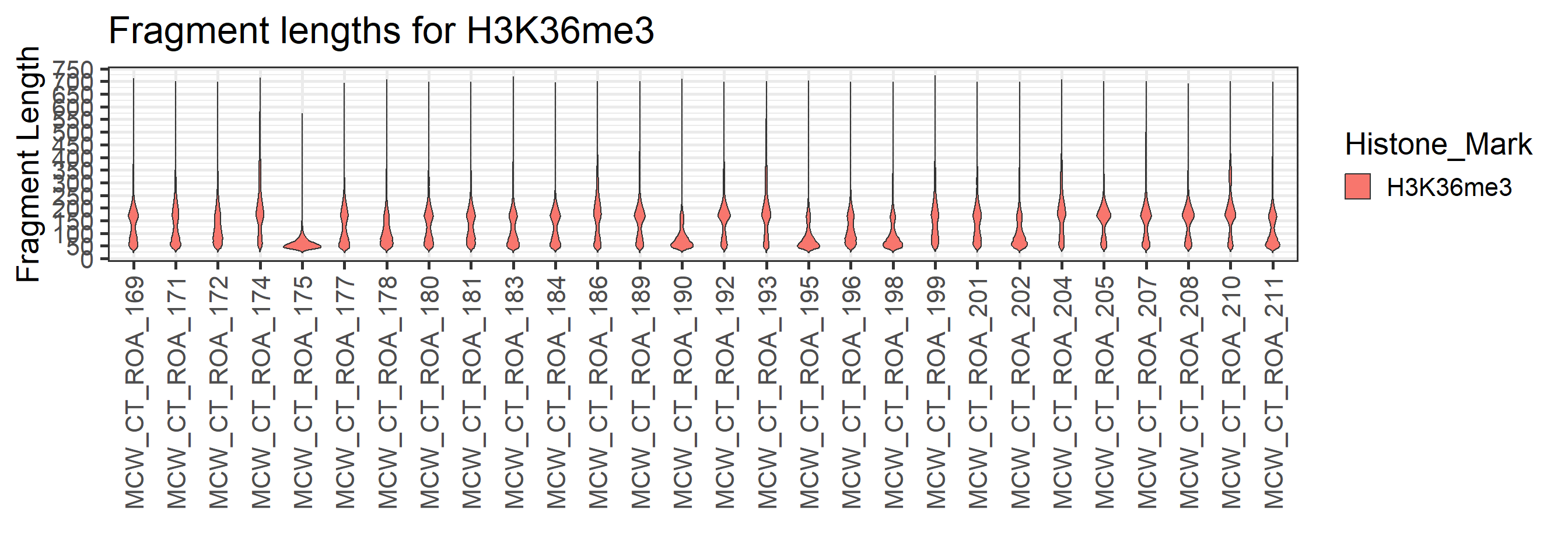
Tagging Questionable Libraries by Frag Len
peaks <- data.frame(sample = unique(annotated_noM_df$sample))
peaks[,"peakNum"] <- NA
for (s in peaks$sample) {
  weights <- annotated_combo_df %>%
    dplyr::filter(sample==s) %>%
    dplyr::select(Col1, weight)
  weights$smooth <- smooth_data(x = weights$Col1, y = weights$weight, sm_method = "moving-average", window_width_n = 15)
  weights$peak <- ggpmisc::find_peaks(weights$smooth, span = 31, global.threshold = 0.01)
  peaks[peaks$sample == s,"peakNum"] <- sum(as.numeric(weights$peak[-1:-150]))
}
questionable_frag_filter = peaks[(peaks$peakNum == 0),]
questionable_frag_filter %>%
  left_join(., sampleinfo, by =c("sample"="Library ID")) %>%
  datatable()
# write_delim(peaks,"data/number_frag_peaks_summary.txt",delim="\t")
sessionInfo()R version 4.4.2 (2024-10-31 ucrt)
Platform: x86_64-w64-mingw32/x64
Running under: Windows 11 x64 (build 26200)
Matrix products: default
locale:
[1] LC_COLLATE=English_United States.utf8
[2] LC_CTYPE=English_United States.utf8
[3] LC_MONETARY=English_United States.utf8
[4] LC_NUMERIC=C
[5] LC_TIME=English_United States.utf8
time zone: America/Chicago
tzcode source: internal
attached base packages:
[1] stats4 grid stats graphics grDevices utils datasets
[8] methods base
other attached packages:
[1] gcplyr_1.12.0 ggpmisc_0.6.2
[3] ggpp_0.5.9 corrplot_0.95
[5] ggpubr_0.6.1 DESeq2_1.46.0
[7] SummarizedExperiment_1.36.0 Biobase_2.66.0
[9] MatrixGenerics_1.18.1 matrixStats_1.5.0
[11] chromVAR_1.28.0 GenomicRanges_1.58.0
[13] GenomeInfoDb_1.42.3 IRanges_2.40.1
[15] S4Vectors_0.44.0 BiocGenerics_0.52.0
[17] genomation_1.38.0 kableExtra_1.4.0
[19] DT_0.33 viridis_0.6.5
[21] viridisLite_0.4.2 data.table_1.17.8
[23] ComplexHeatmap_2.22.0 edgeR_4.4.2
[25] limma_3.62.2 lubridate_1.9.4
[27] forcats_1.0.0 stringr_1.5.1
[29] dplyr_1.1.4 purrr_1.1.0
[31] readr_2.1.5 tidyr_1.3.1
[33] tibble_3.3.0 ggplot2_3.5.2
[35] tidyverse_2.0.0 workflowr_1.7.1
loaded via a namespace (and not attached):
[1] splines_4.4.2 later_1.4.2
[3] BiocIO_1.16.0 bitops_1.0-9
[5] R.oo_1.27.1 XML_3.99-0.18
[7] DirichletMultinomial_1.48.0 lifecycle_1.0.4
[9] rstatix_0.7.2 pwalign_1.2.0
[11] doParallel_1.0.17 rprojroot_2.1.1
[13] vroom_1.6.5 MASS_7.3-65
[15] processx_3.8.6 lattice_0.22-7
[17] crosstalk_1.2.2 backports_1.5.0
[19] magrittr_2.0.3 plotly_4.11.0
[21] sass_0.4.10 rmarkdown_2.29
[23] jquerylib_0.1.4 yaml_2.3.10
[25] plotrix_3.8-4 httpuv_1.6.16
[27] DBI_1.2.3 CNEr_1.42.0
[29] RColorBrewer_1.1-3 abind_1.4-8
[31] zlibbioc_1.52.0 R.utils_2.13.0
[33] RCurl_1.98-1.17 git2r_0.36.2
[35] circlize_0.4.16 GenomeInfoDbData_1.2.13
[37] seqLogo_1.72.0 MatrixModels_0.5-4
[39] annotate_1.84.0 svglite_2.2.1
[41] codetools_0.2-20 DelayedArray_0.32.0
[43] xml2_1.4.0 tidyselect_1.2.1
[45] shape_1.4.6.1 UCSC.utils_1.2.0
[47] farver_2.1.2 GenomicAlignments_1.42.0
[49] jsonlite_2.0.0 GetoptLong_1.0.5
[51] Formula_1.2-5 survival_3.8-3
[53] iterators_1.0.14 systemfonts_1.2.3
[55] foreach_1.5.2 splus2R_1.3-5
[57] tools_4.4.2 TFMPvalue_0.0.9
[59] Rcpp_1.1.0 glue_1.8.0
[61] gridExtra_2.3 SparseArray_1.6.2
[63] xfun_0.52 withr_3.0.2
[65] fastmap_1.2.0 SparseM_1.84-2
[67] callr_3.7.6 caTools_1.18.3
[69] digest_0.6.37 timechange_0.3.0
[71] R6_2.6.1 mime_0.13
[73] seqPattern_1.38.0 textshaping_1.0.1
[75] colorspace_2.1-1 GO.db_3.20.0
[77] gtools_3.9.5 poweRlaw_1.0.0
[79] dichromat_2.0-0.1 RSQLite_2.4.3
[81] R.methodsS3_1.8.2 utf8_1.2.6
[83] generics_0.1.4 rtracklayer_1.66.0
[85] httr_1.4.7 htmlwidgets_1.6.4
[87] S4Arrays_1.6.0 TFBSTools_1.44.0
[89] whisker_0.4.1 pkgconfig_2.0.3
[91] gtable_0.3.6 blob_1.2.4
[93] impute_1.80.0 XVector_0.46.0
[95] htmltools_0.5.8.1 carData_3.0-5
[97] clue_0.3-66 scales_1.4.0
[99] png_0.1-8 knitr_1.50
[101] rstudioapi_0.17.1 tzdb_0.5.0
[103] reshape2_1.4.4 rjson_0.2.23
[105] curl_7.0.0 cachem_1.1.0
[107] GlobalOptions_0.1.2 KernSmooth_2.23-26
[109] parallel_4.4.2 miniUI_0.1.2
[111] AnnotationDbi_1.68.0 restfulr_0.0.16
[113] pillar_1.11.0 vctrs_0.6.5
[115] promises_1.3.3 car_3.1-3
[117] xtable_1.8-4 cluster_2.1.8.1
[119] evaluate_1.0.5 cli_3.6.5
[121] locfit_1.5-9.12 compiler_4.4.2
[123] Rsamtools_2.22.0 rlang_1.1.6
[125] crayon_1.5.3 ggsignif_0.6.4
[127] labeling_0.4.3 ps_1.9.1
[129] getPass_0.2-4 plyr_1.8.9
[131] fs_1.6.6 stringi_1.8.7
[133] gridBase_0.4-7 BiocParallel_1.40.2
[135] Biostrings_2.74.1 lazyeval_0.2.2
[137] quantreg_6.1 Matrix_1.7-3
[139] BSgenome_1.74.0 hms_1.1.3
[141] bit64_4.6.0-1 KEGGREST_1.46.0
[143] statmod_1.5.0 shiny_1.11.1
[145] broom_1.0.9 memoise_2.0.1
[147] bslib_0.9.0 bit_4.6.0
[149] polynom_1.4-1