Examining motif clusters
Renee Matthews
2025-08-25
Last updated: 2026-01-30
Checks: 7 0
Knit directory: DXR_continue/
This reproducible R Markdown analysis was created with workflowr (version 1.7.1). The Checks tab describes the reproducibility checks that were applied when the results were created. The Past versions tab lists the development history.
Great! Since the R Markdown file has been committed to the Git repository, you know the exact version of the code that produced these results.
Great job! The global environment was empty. Objects defined in the global environment can affect the analysis in your R Markdown file in unknown ways. For reproduciblity it’s best to always run the code in an empty environment.
The command set.seed(20250701) was run prior to running
the code in the R Markdown file. Setting a seed ensures that any results
that rely on randomness, e.g. subsampling or permutations, are
reproducible.
Great job! Recording the operating system, R version, and package versions is critical for reproducibility.
Nice! There were no cached chunks for this analysis, so you can be confident that you successfully produced the results during this run.
Great job! Using relative paths to the files within your workflowr project makes it easier to run your code on other machines.
Great! You are using Git for version control. Tracking code development and connecting the code version to the results is critical for reproducibility.
The results in this page were generated with repository version 0886e0d. See the Past versions tab to see a history of the changes made to the R Markdown and HTML files.
Note that you need to be careful to ensure that all relevant files for
the analysis have been committed to Git prior to generating the results
(you can use wflow_publish or
wflow_git_commit). workflowr only checks the R Markdown
file, but you know if there are other scripts or data files that it
depends on. Below is the status of the Git repository when the results
were generated:
Ignored files:
    Ignored:    .Rhistory
    Ignored:    .Rproj.user/
    Ignored:    data/Bed_exports/
    Ignored:    data/Cormotif_data/
    Ignored:    data/DER_data/
    Ignored:    data/Other_paper_data/
    Ignored:    data/RDS_files/
    Ignored:    data/TE_annotation/
    Ignored:    data/alignment_summary.txt
    Ignored:    data/all_peak_final_dataframe.txt
    Ignored:    data/cell_line_info_.tsv
    Ignored:    data/full_summary_QC_metrics.txt
    Ignored:    data/motif_lists/
    Ignored:    data/number_frag_peaks_summary.txt

Untracked files:
    Untracked:  H3K27ac_all_regions_test.bed
    Untracked:  H3K27ac_consensus_clusters_test.bed
    Untracked:  analysis/ATAC_integration_data1.Rmd
    Untracked:  analysis/GREAT_H3K27ac.Rmd
    Untracked:  analysis/H3K27ac_ChromHMM_FC.Rmd
    Untracked:  analysis/H3K27ac_TE_investigation.Rmd
    Untracked:  analysis/H3K27ac_cisRE.Rmd
    Untracked:  analysis/H3K27me3_TE_investigation.Rmd
    Untracked:  analysis/H3K36me3_TE_investigation.Rmd
    Untracked:  analysis/H3K9me3_TE_investigation.Rmd
    Untracked:  analysis/Top2a_Top2b_expression.Rmd
    Untracked:  analysis/dual_histone_TE_investigation.Rmd
    Untracked:  analysis/maps_and_plots.Rmd
    Untracked:  analysis/proteomics.Rmd
    Untracked:  other_analysis/

Unstaged changes:
    Modified:   analysis/H3K27ac_RNA_integration.Rmd
    Modified:   analysis/H3K27ac_TF_motifs.Rmd
    Modified:   analysis/chromHMM.Rmd
    Modified:   analysis/final_analysis.Rmd
    Modified:   analysis/summit_files_processing.Rmd
Note that any generated files, e.g. HTML, png, CSS, etc., are not included in this status report because it is ok for generated content to have uncommitted changes.
These are the previous versions of the repository in which changes were
made to the R Markdown
(analysis/Motif_cluster_analysis.Rmd) and HTML
(docs/Motif_cluster_analysis.html) files. If you’ve
configured a remote Git repository (see ?wflow_git_remote),
click on the hyperlinks in the table below to view the files as they
were in that past version.
| File | Version | Author | Date | Message |
|---|---|---|---|---|
| Rmd | 0886e0d | reneeisnowhere | 2026-01-30 | adding in stats and counts |
| Rmd | 916fa97 | reneeisnowhere | 2026-01-30 | wflow_publish("analysis/Motif_cluster_analysis.Rmd") |
| html | 95e92c1 | reneeisnowhere | 2026-01-20 | Build site. |
| Rmd | aecae6b | reneeisnowhere | 2026-01-20 | wflow_git_commit("analysis/Motif_cluster_analysis.Rmd") |
| Rmd | d85bc60 | reneeisnowhere | 2026-01-15 | wflow_git_commit(c("analysis/H3K9me3_summit_processing.Rmd", |
| html | 1ce5e71 | reneeisnowhere | 2025-09-16 | Build site. |
| Rmd | 911d5b0 | reneeisnowhere | 2025-09-16 | wflow_publish("analysis/Motif_cluster_analysis.Rmd") |
| html | 1a7940a | reneeisnowhere | 2025-09-03 | Build site. |
| Rmd | c572b2b | reneeisnowhere | 2025-09-03 | wflow_publish("analysis/Motif_cluster_analysis.Rmd") |
library(tidyverse)
library(readr)
library(edgeR)
library(ComplexHeatmap)
library(data.table)
library(dplyr)
library(stringr)
library(ggplot2)
library(viridis)
library(DT)
library(kableExtra)
library(genomation)
library(GenomicRanges)
library(ggpubr) ## For customizing figures
library(corrplot) ## For correlation plot
library(ggpmisc)
library(gcplyr)
library(Rsubread)
library(limma)
library(ggrastr)
library(cowplot)
library(smplot2)
library(ggVennDiagram)
library(ggsignif)
library(BiocParallel)
library(TxDb.Hsapiens.UCSC.hg38.knownGene)
library(ChIPseeker)
# sampleinfo <- read_delim("data/sample_info.tsv", delim = "\t")
H3K27ac_set1 <- read_delim("data/motif_lists/H3K27ac_set1.txt",delim="\t")
H3K27ac_set2 <- read_delim("data/motif_lists/H3K27ac_set2.txt",delim="\t")
H3K27ac_set3 <- read_delim("data/motif_lists/H3K27ac_set3.txt",delim="\t")
H3K27me3_set1 <- read_delim("data/motif_lists/H3K27me3_set1.txt",delim="\t")
H3K27me3_set2 <- read_delim("data/motif_lists/H3K27me3_set2.txt",delim="\t")
H3K36me3_set1 <- read_delim("data/motif_lists/H3K36me3_set1.txt",delim="\t")
H3K36me3_set2 <- read_delim("data/motif_lists/H3K36me3_set2.txt",delim="\t")
H3K9me3_set1 <- read_delim("data/motif_lists/H3K9me3_set1.txt",delim="\t")
H3K9me3_set2 <- read_delim("data/motif_lists/H3K9me3_set2.txt",delim="\t")
H3K9me3_set3 <- read_delim("data/motif_lists/H3K9me3_set3.txt",delim="\t")
### loading filtered raw counts for visualization
H3K27ac_filt_raw_counts <- read_delim("data/DER_data/H3K27ac_filtered_raw_counts.txt",delim = "\t") %>% column_to_rownames("Peakid")
H3K27me3_filt_raw_counts <- read_delim("data/DER_data/H3K27me3_filtered_raw_counts.txt",delim = "\t")%>% column_to_rownames("Peakid")
H3K36me3_filt_raw_counts <- read_delim("data/DER_data/H3K36me3_filtered_raw_counts.txt",delim = "\t")%>% column_to_rownames("Peakid")
H3K9me3_filt_raw_counts <- read_delim( "data/DER_data/H3K9me3_filtered_raw_counts.txt",delim = "\t")%>% column_to_rownames("Peakid")
all_H3K27ac_regions <- H3K27ac_filt_raw_counts %>% rownames_to_column("Peakid") %>% distinct(Peakid)
all_H3K27me3_regions <- H3K27me3_filt_raw_counts %>% rownames_to_column("Peakid") %>% distinct(Peakid)
all_H3K36me3_regions <- H3K36me3_filt_raw_counts %>% rownames_to_column("Peakid") %>% distinct(Peakid)
all_H3K9me3_regions <- H3K9me3_filt_raw_counts %>% rownames_to_column("Peakid") %>% distinct(Peakid)
H3K27ac_filt_lcpm <- cpm(H3K27ac_filt_raw_counts, log = TRUE)
H3K27me3_filt_lcpm <- cpm(H3K27me3_filt_raw_counts, log = TRUE)
H3K36me3_filt_lcpm <- cpm(H3K36me3_filt_raw_counts, log = TRUE)
H3K9me3_filt_lcpm <- cpm(H3K9me3_filt_raw_counts, log = TRUE)
H3K9me3_toplist <- readRDS( "data/DER_data/H3K9me3_toplist_nooutlier.RDS")
H3K36me3_toplist <- readRDS( "data/DER_data/H3K36me3_toplist_nooutlier.RDS")
H3K27me3_toplist <- readRDS( "data/DER_data/H3K27me3_toplist.RDS")
H3K27ac_toplist <- readRDS( "data/DER_data/H3K27ac_toplist.RDS")
H3K27ac_toptable_list <- bind_rows(H3K27ac_toplist, .id = "group")
H3K27me3_toptable_list <- bind_rows(H3K27me3_toplist, .id = "group")
H3K36me3_toptable_list <- bind_rows(H3K36me3_toplist, .id = "group")
H3K9me3_toptable_list <- bind_rows(H3K9me3_toplist, .id = "group")standardizeAnnoList <- function(annoList, categories, color_pal = NULL) {
if (is.null(color_pal)) {
if (!requireNamespace("RColorBrewer", quietly = TRUE)) {
stop("Please install RColorBrewer to use the default palette")
}
color_pal <- RColorBrewer::brewer.pal(length(categories), "Set3")
names(color_pal) <- categories
}
for (nm in names(annoList)) {
annoStat <- annoList[[nm]]@annoStat
# pad missing categories
missing_cats <- setdiff(categories, as.character(annoStat$Feature))
if (length(missing_cats) > 0) {
pad <- data.frame(Feature = missing_cats, Frequency = 0)
annoStat <- rbind(annoStat, pad)
}
# factor + reorder rows
annoStat$Feature <- factor(annoStat$Feature, levels = categories)
annoStat <- annoStat[order(match(annoStat$Feature, categories)), ]
annoList[[nm]]@annoStat <- annoStat
}
return(list(
annoList = annoList,
color_pal = color_pal
))
}H3K27ac motifs samples
Set 1
examp_H3K27ac_1 <-#slice_sample(H3K27ac_set1,n = 3, replace=FALSE)
    c("chr1:77923740-77924468","chr20:25484622-25485357","chr1:229148017-229149226")
examp_H3K27ac_2 <-#slice_sample(H3K27ac_set2,n = 3, replace=FALSE)
  c("chr5:85451856-85453893","chr10:114271262-114272616", "chr3:63343167-63344341" )
examp_H3K27ac_3 <- #slice_sample(H3K27ac_set3,n = 3, replace=FALSE)
  c("chr8:8664034-8666371","chr3:141152796-141154087","chr21:43701994-43704465")


H3K27ac_filt_lcpm %>%
  as.data.frame() %>%
   rownames_to_column("Peakid") %>%
  dplyr::filter(Peakid %in% examp_H3K27ac_1) %>%
  ###pivot and add additional information from dataframe
  pivot_longer(., cols = !Peakid, names_to = "sample", values_to = "lcpm" ) %>%
  separate_wider_delim(., cols=sample, delim="_", names=c("ind","tx","time")) %>%
  mutate(ind=factor(ind, levels=c("Ind1", "Ind2", "Ind3", "Ind4","Ind5")),
         tx=factor(tx,levels = c("DOX","VEH")),
         time=factor(time, levels=c("24T","24R","144R")),
         group_graph= paste0(tx, "_", time),
         group=paste0("H3K27ac_",time),
      group_graph = factor(group_graph, levels = c(
        "DOX_24T",  "VEH_24T",
        "DOX_24R",  "VEH_24R",
        "DOX_144R",  "VEH_144R"))) %>%

  ggplot(., aes(x=group_graph, y=lcpm)) +
  geom_boxplot(aes(fill=tx))+
  facet_wrap(~Peakid, scales="free")+
  theme_bw()+
  theme(axis.text.x=element_text(angle = 90))+
  ggtitle("set 1 H3K27ac samples")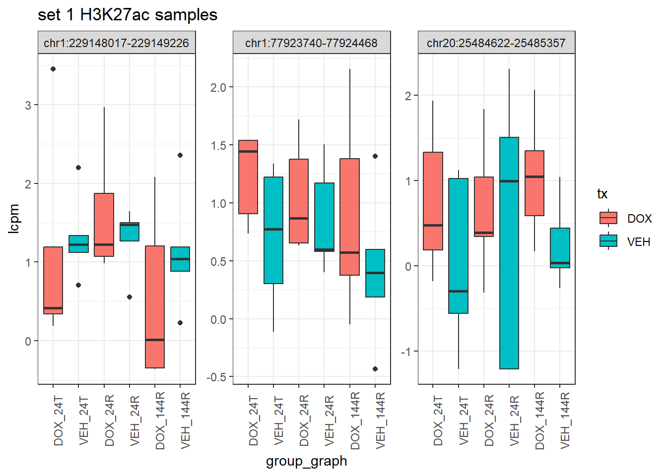
| Version | Author | Date |
|---|---|---|
| 1a7940a | reneeisnowhere | 2025-09-03 |
Set 2
H3K27ac_filt_lcpm %>%
  as.data.frame() %>%
  dplyr::filter(row.names(H3K27ac_filt_lcpm) %in% examp_H3K27ac_2) %>%
  ###pivot and add additional information from dataframe
  rownames_to_column("Peakid") %>%
  pivot_longer(., cols = !Peakid, names_to = "sample", values_to = "lcpm" ) %>%
  separate_wider_delim(., cols=sample, delim="_", names=c("ind","tx","time")) %>%
  mutate(ind=factor(ind, levels=c("Ind1", "Ind2", "Ind3", "Ind4","Ind5")),
         tx=factor(tx,levels = c("DOX","VEH")),
         time=factor(time, levels=c("24T","24R","144R")),
         group_graph= paste0(tx, "_", time),
         group=paste0("H3K27ac_",time),
      group_graph = factor(group_graph, levels = c(
        "DOX_24T",  "VEH_24T",
        "DOX_24R",  "VEH_24R",
        "DOX_144R",  "VEH_144R"))) %>%

  ggplot(., aes(x=group_graph, y=lcpm)) +
  geom_boxplot(aes(fill=tx))+
  facet_wrap(~Peakid, scales="free")+
  theme_bw()+
  theme(axis.text.x=element_text(angle = 90))+
  ggtitle("set 2 H3K27ac samples")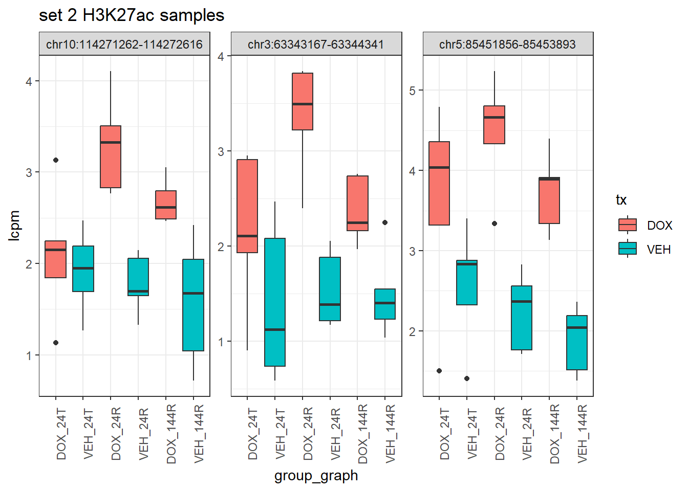
| Version | Author | Date |
|---|---|---|
| 1a7940a | reneeisnowhere | 2025-09-03 |
Set 3
H3K27ac_filt_lcpm %>%
  as.data.frame() %>%
  dplyr::filter(row.names(H3K27ac_filt_lcpm) %in% examp_H3K27ac_3) %>%
  ###pivot and add additional information from dataframe
  rownames_to_column("Peakid") %>%
  pivot_longer(., cols = !Peakid, names_to = "sample", values_to = "lcpm" ) %>%
  separate_wider_delim(., cols=sample, delim="_", names=c("ind","tx","time")) %>%
  mutate(ind=factor(ind, levels=c("Ind1", "Ind2", "Ind3", "Ind4","Ind5")),
         tx=factor(tx,levels = c("DOX","VEH")),
         time=factor(time, levels=c("24T","24R","144R")),
         group_graph= paste0(tx, "_", time),
         group=paste0("H3K27ac_",time),
      group_graph = factor(group_graph, levels = c(
        "DOX_24T",  "VEH_24T",
        "DOX_24R",  "VEH_24R",
        "DOX_144R",  "VEH_144R"))) %>%

  ggplot(., aes(x=group_graph, y=lcpm)) +
  geom_boxplot(aes(fill=tx))+
  facet_wrap(~Peakid, scales="free")+
  theme_bw()+
  theme(axis.text.x=element_text(angle = 90))+
  ggtitle("set 3 H3K27ac samples")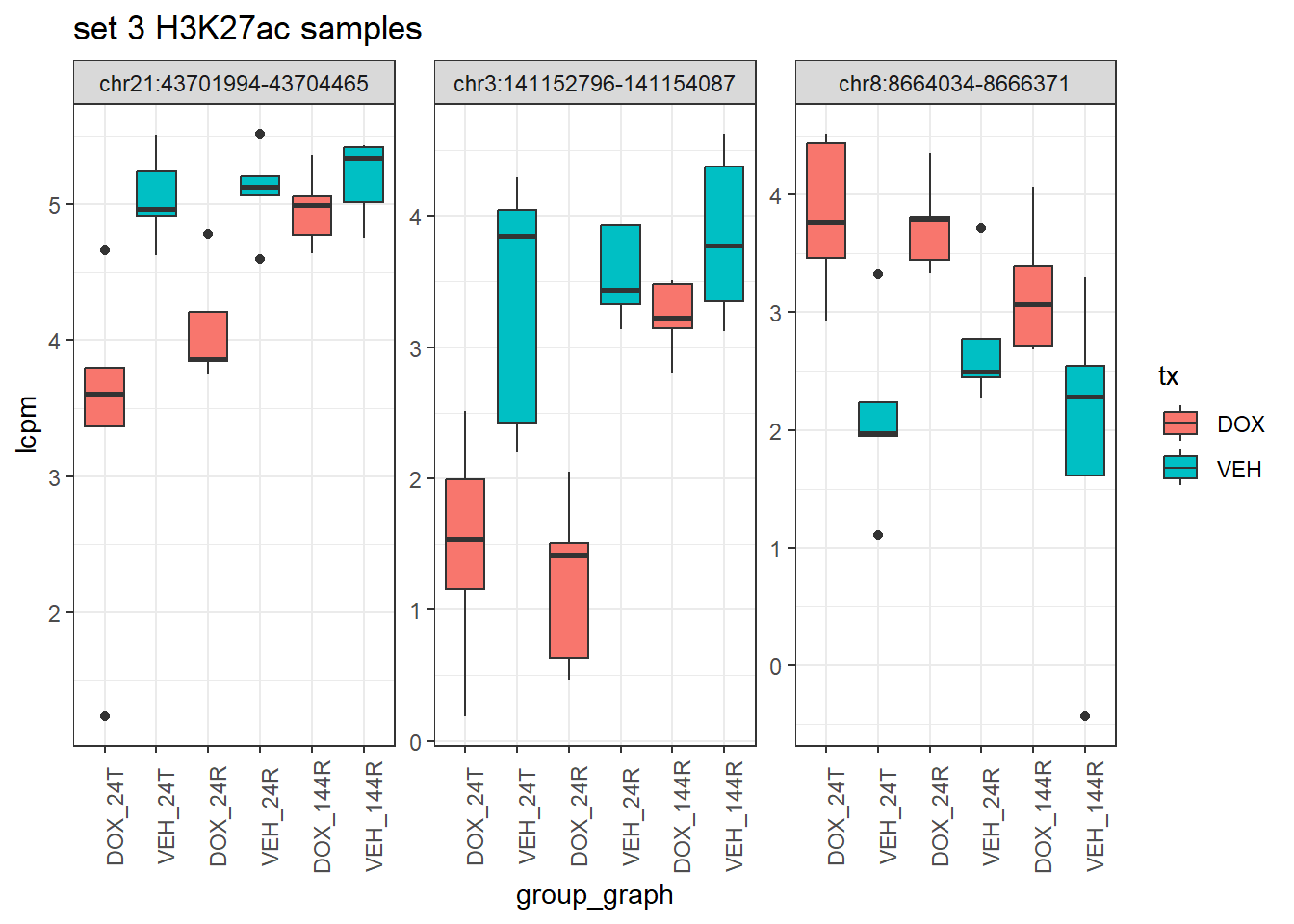
| Version | Author | Date |
|---|---|---|
| 1a7940a | reneeisnowhere | 2025-09-03 |
Genomic regions
txdb <- TxDb.Hsapiens.UCSC.hg38.knownGene

all_H3K27ac_regions_gr <- all_H3K27ac_regions %>%
    tidyr::separate(., col = "Peakid", into=c("seqnames","range"), sep = ":", remove=FALSE) %>%
  tidyr::separate(., col = "range", into=c("start","end"), sep = "-") %>%
  GRanges()


H3K27ac_set1_gr <- H3K27ac_set1 %>%
  tidyr::separate(., col = ".", into=c("seqnames","range"), sep = ":", remove=FALSE) %>%
  tidyr::separate(., col = "range", into=c("start","end"), sep = "-") %>%
  dplyr::rename("Peakid"=".") %>%
  GRanges()

H3K27ac_set2_gr <- H3K27ac_set2 %>%
  tidyr::separate(., col = ".", into=c("seqnames","range"), sep = ":", remove=FALSE) %>%
  tidyr::separate(., col = "range", into=c("start","end"), sep = "-") %>%
  dplyr::rename("Peakid"=".") %>%
  GRanges()

H3K27ac_set3_gr <- H3K27ac_set3 %>%
  tidyr::separate(., col = ".", into=c("seqnames","range"), sep = ":", remove=FALSE) %>%
  tidyr::separate(., col = "range", into=c("start","end"), sep = "-") %>%
  dplyr::rename("Peakid"=".") %>%
  GRanges()
H3K27ac_list <- list("Set_1"=H3K27ac_set1_gr,"Set_2"=H3K27ac_set2_gr,"Set_3"=H3K27ac_set3_gr,"all_H3K27ac"=all_H3K27ac_regions_gr)


# peakAnnoList_H3K27ac <- lapply(H3K27ac_list, annotatePeak, tssRegion =c(-2000,2000), TxDb=txdb)

# saveRDS(peakAnnoList_H3K27ac, "data/motif_lists/H3K27ac_annotated_peaks.RDS")
peakAnnoList_H3K27ac <- readRDS("data/motif_lists/H3K27ac_annotated_peaks.RDS")

categories <- c(
  "Distal Intergenic", "Downstream (<=300)",
  "Other Intron", "1st Intron",
  "Other Exon", "1st Exon",
  "3' UTR", "5' UTR",
  "Promoter (1-2kb)", "Promoter (<=1kb)"
)

# Optional: custom color palette
color_pal <- c(
  "#6a3d9a", "#cab2d6",
  "#ff7f00", "#fdbf6f",
  "#e31a1c", "#fb9a99",
  "#33a02c", "#b2df8a",
  "#1f78b4", "#a6cee3"
)
names(color_pal) <- categories

res <- standardizeAnnoList(peakAnnoList_H3K27ac, categories, color_pal)
peakAnnoList_H3K27ac_std <- res$annoList
color_pal_std <- res$color_pal

# bar plot
plotAnnoBar(peakAnnoList_H3K27ac_std[c(4,1,2,3)]) +
  scale_fill_manual(values=color_pal_std) +
  ggtitle("H3K27ac Feature Distribution")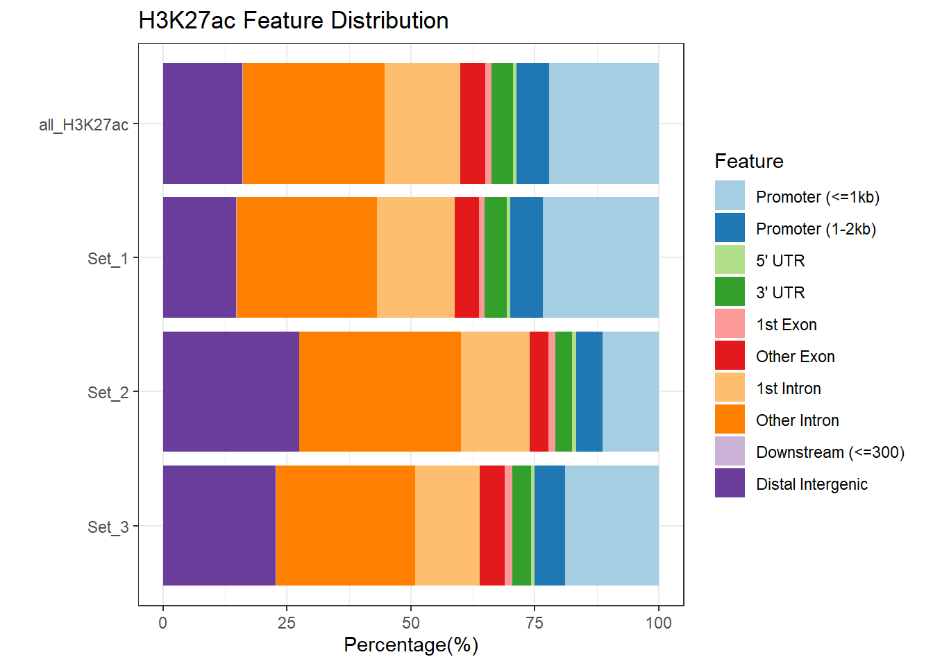
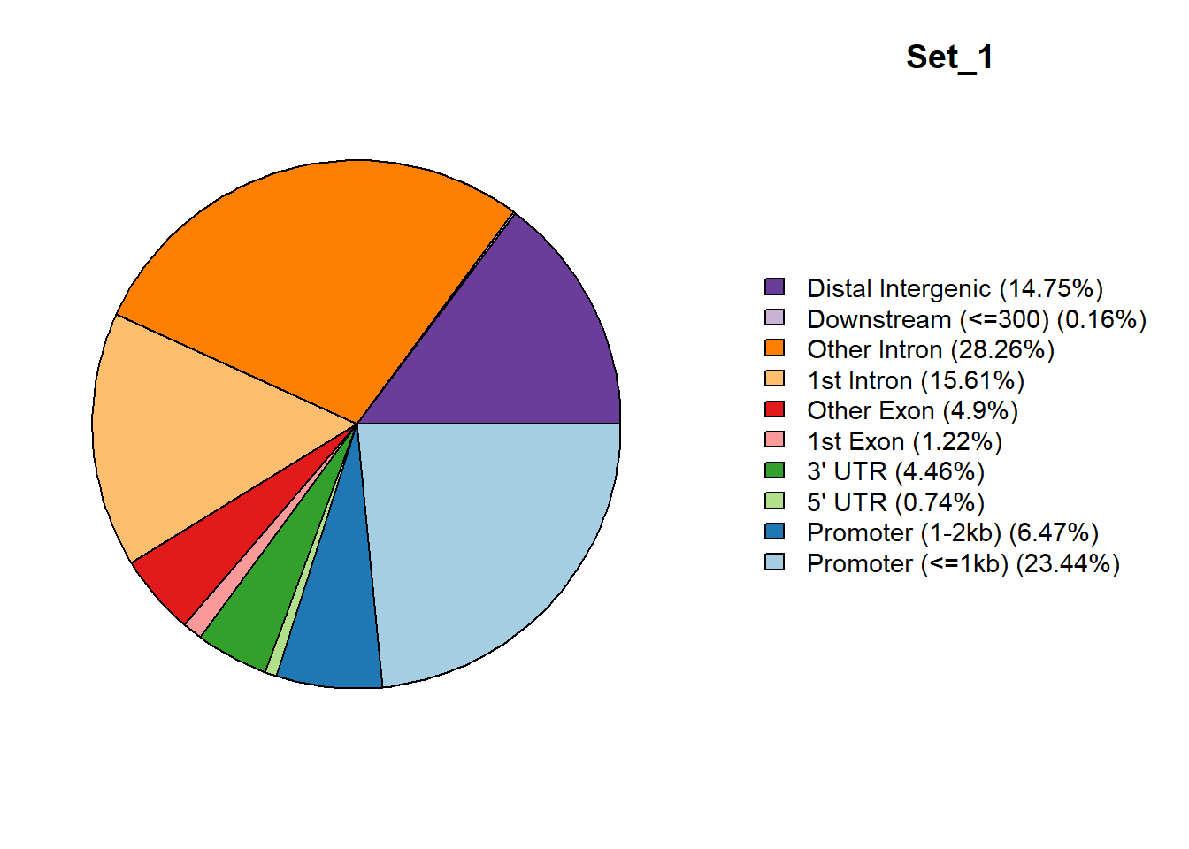
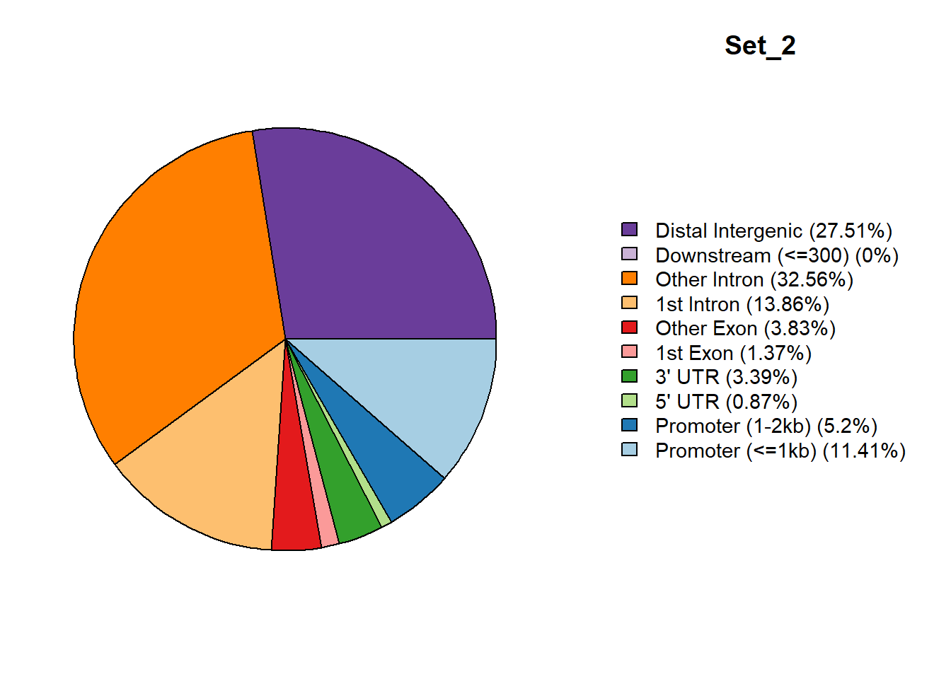
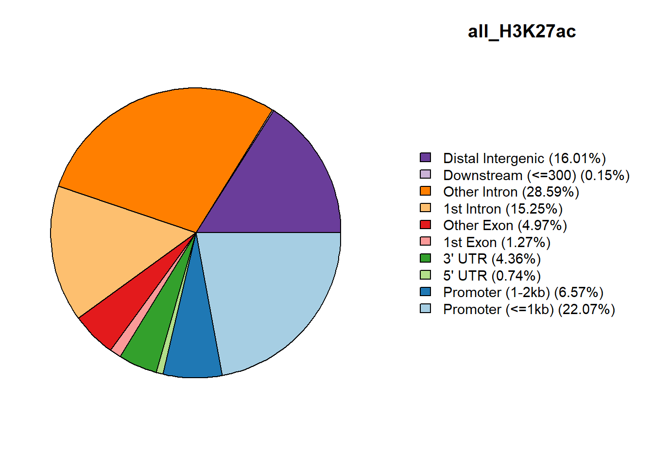
# pie plots
for (nm in names(peakAnnoList_H3K27ac_std)) {
  plotAnnoPie(peakAnnoList_H3K27ac_std[[nm]], col=color_pal_std)
  title(main = nm, line = -2)
}

Histone proportions
H3K27ac_lookup <- imap_dfr(peakAnnoList_H3K27ac[1:3], ~
  tibble(Peakid = .x@anno$Peakid, cluster = .y))
all_H3K27ac_regions %>%
  mutate(group="H3K27ac") %>%
  left_join(., H3K27ac_lookup) %>%
   tidyr::replace_na(list(cluster = "NA")) %>%
  ggplot(., aes(y=group,fill=cluster))+
  geom_bar()+
  geom_text(aes( label = scales::percent(..prop..),
                   x= ..prop.. ), stat= "count", vjust = -.5)+
  ggtitle("H3K27ac proportions of ROIs")+
  theme_classic()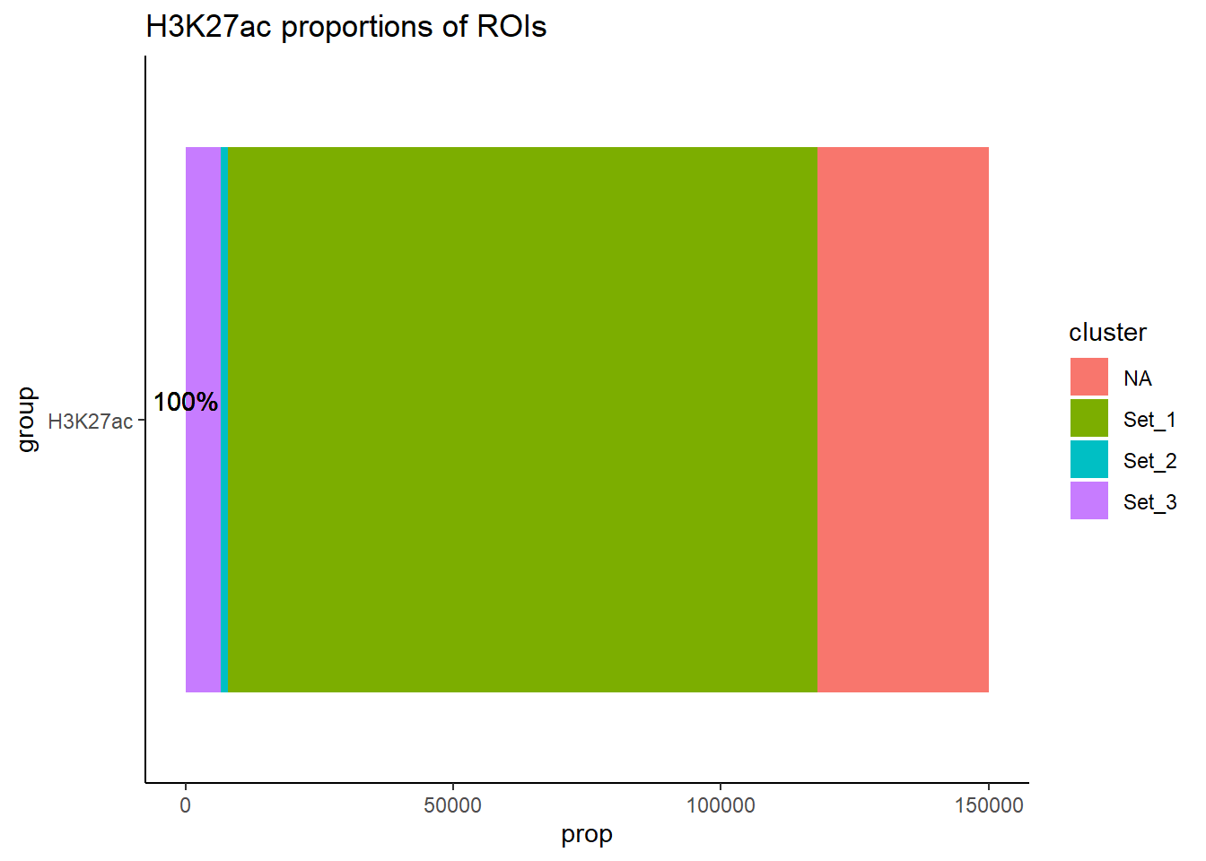
all_H3K27ac_regions %>%
  mutate(group="H3K27ac") %>%
  left_join(., H3K27ac_lookup) %>%
   tidyr::replace_na(list(cluster = "NA")) %>%
  mutate(cluster=factor(cluster, levels = c("Set_1","Set_2","Set_3","NA"))) %>%
  ggplot(., aes(x=cluster,y = after_stat(prop),fill=cluster, group=1))+
  geom_bar(aes(stat="count"))+
  geom_text(aes( label = scales::percent(after_stat(prop))),
            stat= "count", vjust = -.5)+
  scale_y_continuous(
    labels = scales::percent,
    expand = expansion(mult = c(0, 0.1))
  ) +
  ggtitle("H3K27ac proportions of ROIs")+
  theme_classic()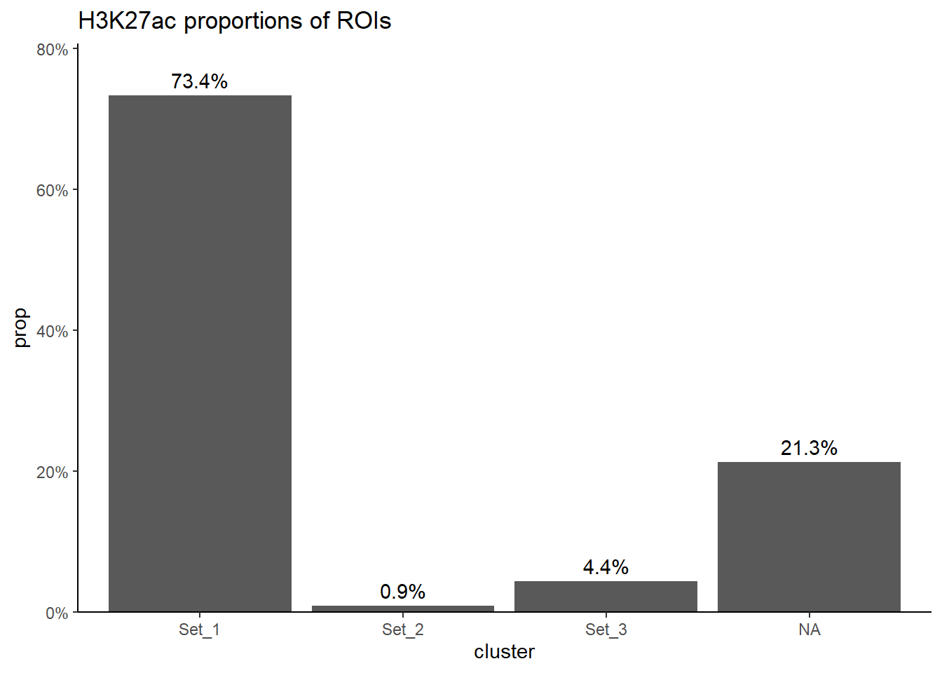
all_H3K27ac_regions %>%
  mutate(group="H3K27ac") %>%
  left_join(., H3K27ac_lookup) %>%
   tidyr::replace_na(list(cluster = "NA")) %>%
  group_by(cluster) %>%
  tally(name = "n_ROIs") %>%
  ungroup() %>%
  DT::datatable(
    rownames = FALSE,
    caption = htmltools::tags$caption(
      style = "caption-side: top; text-align: left;",
      "H3K27ac ROI counts per cluster"
    ),
    options = list(
      pageLength = 10,
      autoWidth = TRUE,
      dom = "tip"
    )
  )
LFC H3K27ac
Set1
# H3K27ac_toptable_list %>%
#   dplyr::filter(genes %in% H3K27ac_set1$.) %>%
#   dplyr::select(group,genes,logFC) %>%
#   mutate(group=factor(group, levels = c("H3K27ac_24T","H3K27ac_24R","H3K27ac_144R"))) %>%
#   ggplot(., aes(x=group, y=logFC))+
#   geom_boxplot(aes(fill=group))+
#   geom_signif(comparisons = list(c("H3K27ac_24T", "H3K27ac_144R"),
#                                  c("H3K27ac_24T","H3K27ac_24R"),
#                                  c("H3K27ac_24R", "H3K27ac_144R")),
#                               step_increase = 0.1,
#               map_signif_level = FALSE,
#               test = "wilcox.test")+
#   theme_bw()+
#   ggtitle("LFC across time for H3K27ac set1")


H3K27ac_toptable_list %>%
  dplyr::filter(genes %in% H3K27ac_set1$.) %>%
  dplyr::select(group,genes,logFC) %>%
  mutate(group=factor(group, levels = c("H3K27ac_24T","H3K27ac_24R","H3K27ac_144R")),
         logFC=abs(logFC)) %>%
  ggplot(., aes(x=group, y=logFC))+
  geom_boxplot(aes(fill=group))+
  geom_signif(comparisons = list(c("H3K27ac_24T", "H3K27ac_144R"),
                                 c("H3K27ac_24T","H3K27ac_24R"),
                                 c("H3K27ac_24R", "H3K27ac_144R")),
                              step_increase = 0.1,
              map_signif_level = FALSE,
              test = "wilcox.test")+
  theme_bw()+
  ggtitle("Absolute LFC across time for H3K27ac set1")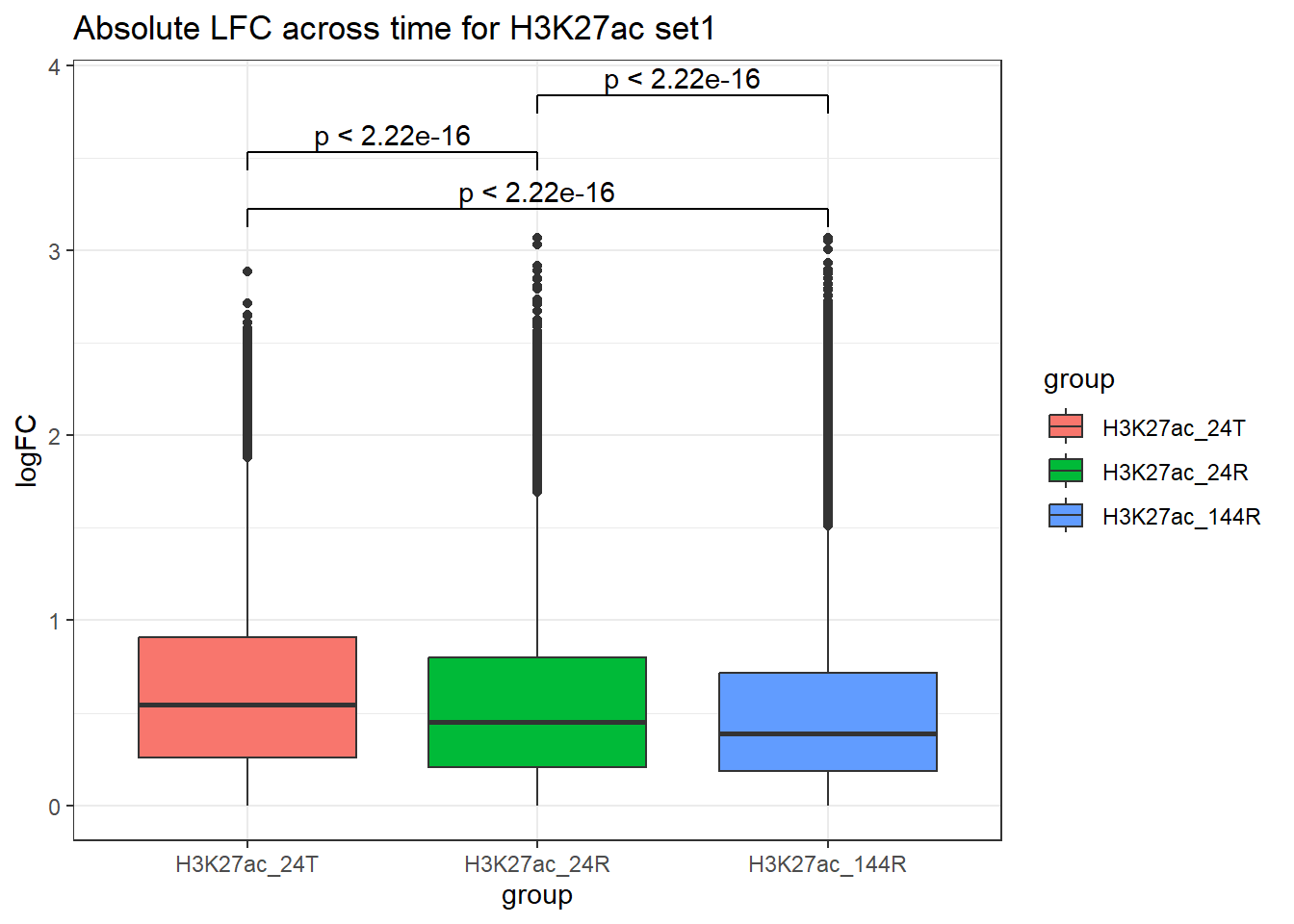
| Version | Author | Date |
|---|---|---|
| 1a7940a | reneeisnowhere | 2025-09-03 |
  set1_27ac <- H3K27ac_toptable_list %>%
  dplyr::filter(genes %in% H3K27ac_set1$.) %>%
  dplyr::select(group,genes,logFC) %>%
   mutate(group=factor(group, levels = c("H3K27ac_24T","H3K27ac_24R","H3K27ac_144R")),
         logFC=abs(logFC)) %>%
  group_by(group) %>%
  summarize(med_Set1=median(logFC),.groups="drop")
set2
# H3K27ac_toptable_list %>%
#   dplyr::filter(genes %in% H3K27ac_set2$.) %>%
#   dplyr::select(group,genes,logFC) %>%
#   mutate(group=factor(group, levels = c("H3K27ac_24T","H3K27ac_24R","H3K27ac_144R"))) %>%
#   ggplot(., aes(x=group, y=logFC))+
#   geom_boxplot(aes(fill=group))+
#   geom_signif(comparisons = list(c("H3K27ac_24T", "H3K27ac_144R"),
#                                  c("H3K27ac_24T","H3K27ac_24R"),
#                                  c("H3K27ac_24R", "H3K27ac_144R")),
#                               step_increase = 0.1,
#               map_signif_level = FALSE,
#               test = "wilcox.test")+
#   theme_bw()+
#   ggtitle("LFC across time for H3K27ac set2")


H3K27ac_toptable_list %>%
  dplyr::filter(genes %in% H3K27ac_set2$.) %>%
  dplyr::select(group,genes,logFC) %>%
  mutate(group=factor(group, levels = c("H3K27ac_24T","H3K27ac_24R","H3K27ac_144R")),
         logFC=abs(logFC)) %>%
  ggplot(., aes(x=group, y=logFC))+
  geom_boxplot(aes(fill=group))+
  geom_signif(comparisons = list(c("H3K27ac_24T", "H3K27ac_144R"),
                                 c("H3K27ac_24T","H3K27ac_24R"),
                                 c("H3K27ac_24R", "H3K27ac_144R")),
                              step_increase = 0.1,
              map_signif_level = FALSE,
              test = "wilcox.test")+
  theme_bw()+
  ggtitle("Absolute LFC across time for H3K27ac set2")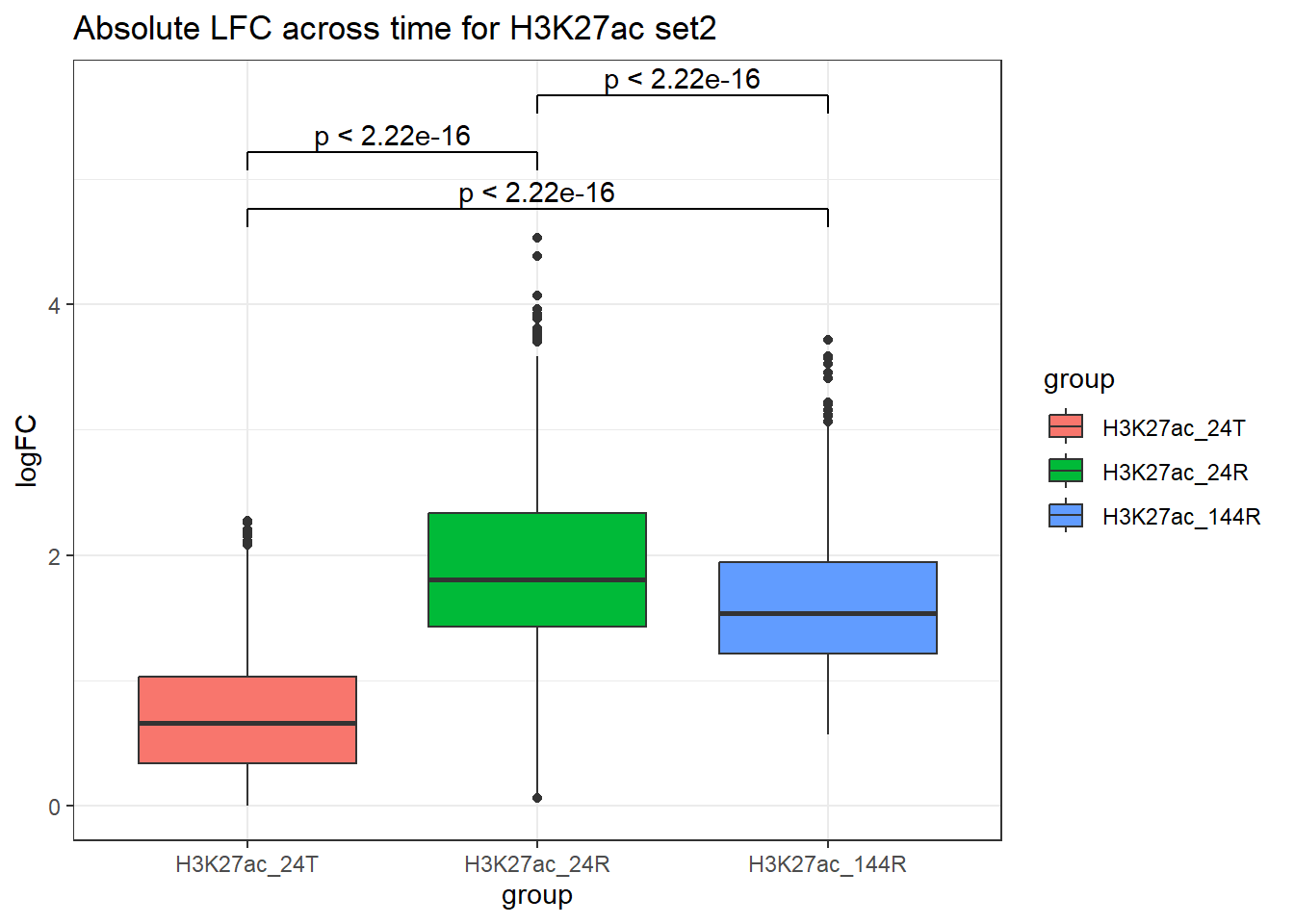
| Version | Author | Date |
|---|---|---|
| 1a7940a | reneeisnowhere | 2025-09-03 |
  set2_27ac <- H3K27ac_toptable_list %>%
  dplyr::filter(genes %in% H3K27ac_set2$.) %>%
  dplyr::select(group,genes,logFC) %>%
   mutate(group=factor(group, levels = c("H3K27ac_24T","H3K27ac_24R","H3K27ac_144R")),
         logFC=abs(logFC)) %>%
  group_by(group) %>%
  summarize(med_Set2=median(logFC),.groups="drop")
set3
# H3K27ac_toptable_list %>%
#   dplyr::filter(genes %in% H3K27ac_set3$.) %>%
#   dplyr::select(group,genes,logFC) %>%
#   mutate(group=factor(group, levels = c("H3K27ac_24T","H3K27ac_24R","H3K27ac_144R"))) %>%
#   ggplot(., aes(x=group, y=logFC))+
#   geom_boxplot(aes(fill=group))+
#   geom_signif(comparisons = list(c("H3K27ac_24T", "H3K27ac_144R"),
#                                  c("H3K27ac_24T","H3K27ac_24R"),
#                                  c("H3K27ac_24R", "H3K27ac_144R")),
#                               step_increase = 0.1,
#               map_signif_level = FALSE,
#               test = "wilcox.test")+
#   theme_bw()+
#   ggtitle("LFC across time for H3K27ac set3")


H3K27ac_toptable_list %>%
  dplyr::filter(genes %in% H3K27ac_set3$.) %>%
  dplyr::select(group,genes,logFC) %>%
  mutate(group=factor(group, levels = c("H3K27ac_24T","H3K27ac_24R","H3K27ac_144R")),
         logFC=abs(logFC)) %>%
  ggplot(., aes(x=group, y=logFC))+
  geom_boxplot(aes(fill=group))+
  geom_signif(comparisons = list(c("H3K27ac_24T", "H3K27ac_144R"),
                                 c("H3K27ac_24T","H3K27ac_24R"),
                                 c("H3K27ac_24R", "H3K27ac_144R")),
                              step_increase = 0.1,
              map_signif_level = FALSE,
              test = "wilcox.test")+
  theme_bw()+
  ggtitle("Absolute LFC across time for H3K27ac set3")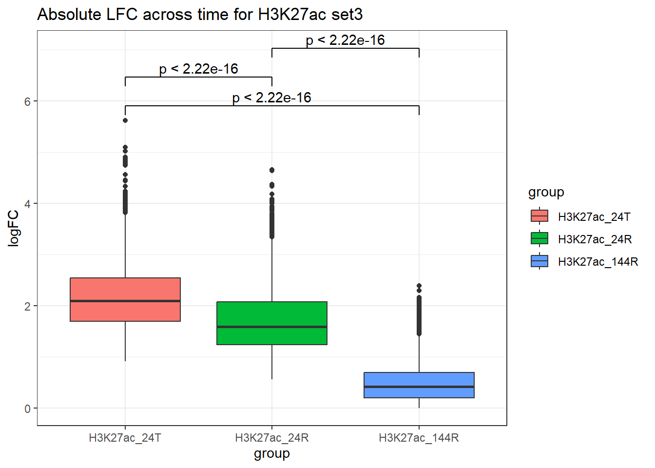
| Version | Author | Date |
|---|---|---|
| 1a7940a | reneeisnowhere | 2025-09-03 |
  H3K27ac_toptable_list %>%
  dplyr::filter(genes %in% H3K27ac_set3$.) %>%
  dplyr::select(group,genes,logFC) %>%
  mutate(group=factor(group, levels = c("H3K27ac_24T","H3K27ac_24R","H3K27ac_144R")),
         logFC=abs(logFC)) %>%
  group_by(group) %>%
  summarize(med_Set3=median(logFC),.groups="drop") %>%
  left_join(set1_27ac, by="group") %>%
  left_join(set2_27ac, by="group") %>%
  pivot_longer(cols=!group, values_to = "median_LFC", names_to = "set") %>%
  ggplot(., aes(x=group, y=median_LFC, group=set, color=set))+
  geom_point(size=4)+
  geom_line(aes(alpha = 0.8, linewidth = 4))+
  theme_bw()+
  ggtitle("LFC across time for H3K27ac sets")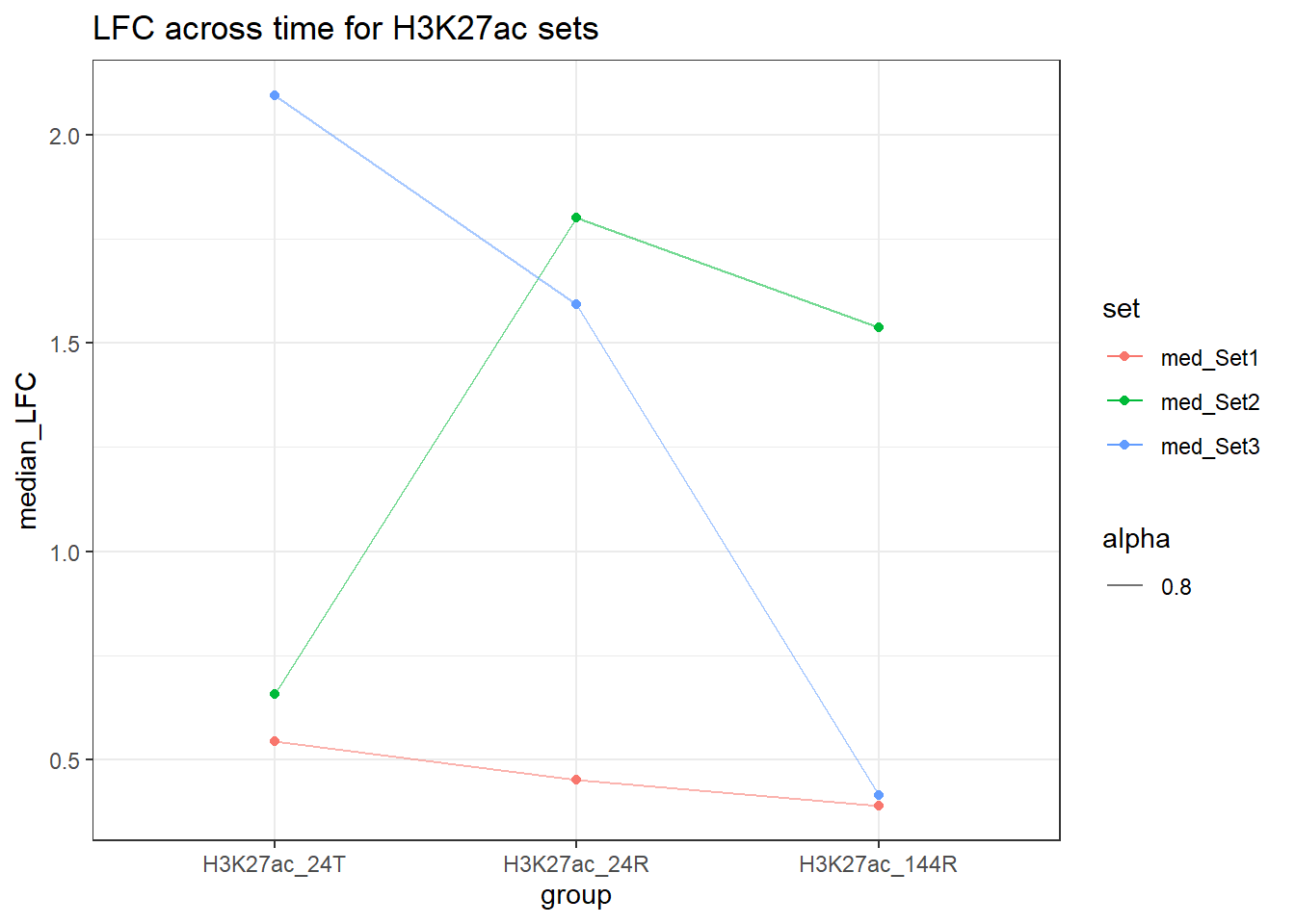
Top 100
This is the calculation of Top 100 in each category, then united
cormotif_initial_H3K27ac <- readRDS("data/Cormotif_data/Cormotif_initial_H3K27ac.RDS")
row.names(cormotif_initial_H3K27ac$bestmotif$clustlike) <- row.names(H3K27ac_filt_lcpm)
H3K27ac_clustlike <- cormotif_initial_H3K27ac$bestmotif$clustlike %>%
  as.data.frame() %>%
  rownames_to_column("Peakid")

H3K27ac_clusters <- list(
  Set1="V1",
  Set2="V2",
  Set3="V3")


Sets_H3K27ac <- H3K27ac_toptable_list %>%
  mutate(cluster=case_when(genes %in% H3K27ac_set1$. ~ "Set1",
                           genes %in% H3K27ac_set2$. ~ "Set2",
                           genes %in% H3K27ac_set3$. ~ "Set3",
                           TRUE ~ "not_assigned")) %>%
  left_join(., H3K27ac_clustlike,by=c("genes"="Peakid")) %>%
  dplyr::filter(cluster!="not_assigned")

###This code uses the H3K27ac_clusters list and filters through Sets_H3K27ac data frame by selecting
Sets_H3K27ac_top <- map_dfr(names(H3K27ac_clusters), function(cl) {
  col <- H3K27ac_clusters[[cl]]
  Sets_H3K27ac %>%
    filter(cluster == cl) %>%
    # group_by(group) %>%
    slice_max(order_by = .data[[col]], n = 100)
}) %>%
  ungroup()

## now plot

Sets_H3K27ac_top %>%
  mutate(group=factor(group, levels = c("H3K27ac_24T","H3K27ac_24R","H3K27ac_144R")),
         cluster=factor(cluster, levels=c("Set1","Set2","Set3"))) %>%
  ggplot(., aes(x= group,y = logFC, group = interaction(cluster, genes), color=cluster))+
  geom_point()+
  geom_line(aes(alpha = 0.8))+
  theme_bw()+
  facet_wrap(~cluster)+
  ggtitle("LFC across time for H3K27ac top 100 by Set")+
  theme(axis.text.x = element_text(angle=90) )
| Version | Author | Date |
|---|---|---|
| 1ce5e71 | reneeisnowhere | 2025-09-16 |
# saveRDS(Sets_H3K27ac_top,"data/motif_lists/H3K27ac_toplistbymotif.RDS")H3K27me3 motifs samples
Set 1
# slice_sample(H3K27me3_set2,n = 3, replace=FALSE)
examp_H3K27me3_1 <-#slice_sample(H3K27me3_set1,n = 3, replace=FALSE)
  c("chr17:8878023-8878923", "chr2:23436468-23436797","chr10:132830096-132830712")
examp_H3K27me3_2 <-#slice_sample(H3K27me3_set2,n = 3, replace=FALSE)
  c("chr5:141004122-141004627" ,  "chr6:101195726-101195968",  "chr3:139117155-139117784")


H3K27me3_filt_lcpm %>%
  as.data.frame() %>%
  dplyr::filter(row.names(H3K27me3_filt_lcpm) %in% examp_H3K27me3_1) %>%
  ###pivot and add additional information from dataframe
  rownames_to_column("Peakid") %>%
  pivot_longer(., cols = !Peakid, names_to = "sample", values_to = "lcpm" ) %>%
  separate_wider_delim(., cols=sample, delim="_", names=c("ind","tx","time")) %>%
  mutate(ind=factor(ind, levels=c("Ind1", "Ind2", "Ind3", "Ind4","Ind5")),
         tx=factor(tx,levels = c("DOX","VEH")),
         time=factor(time, levels=c("24T","24R","144R")),
         group_graph= paste0(tx, "_", time),
         group=paste0("H3K27me3_",time),
      group_graph = factor(group_graph, levels = c(
        "DOX_24T",  "VEH_24T",
        "DOX_24R",  "VEH_24R",
        "DOX_144R",  "VEH_144R"))) %>%

  ggplot(., aes(x=group_graph, y=lcpm)) +
  geom_boxplot(aes(fill=tx))+
  facet_wrap(~Peakid, scales="free")+
  theme_bw()+
  theme(axis.text.x=element_text(angle = 90))+
  ggtitle("set 1 H3K27me3 samples")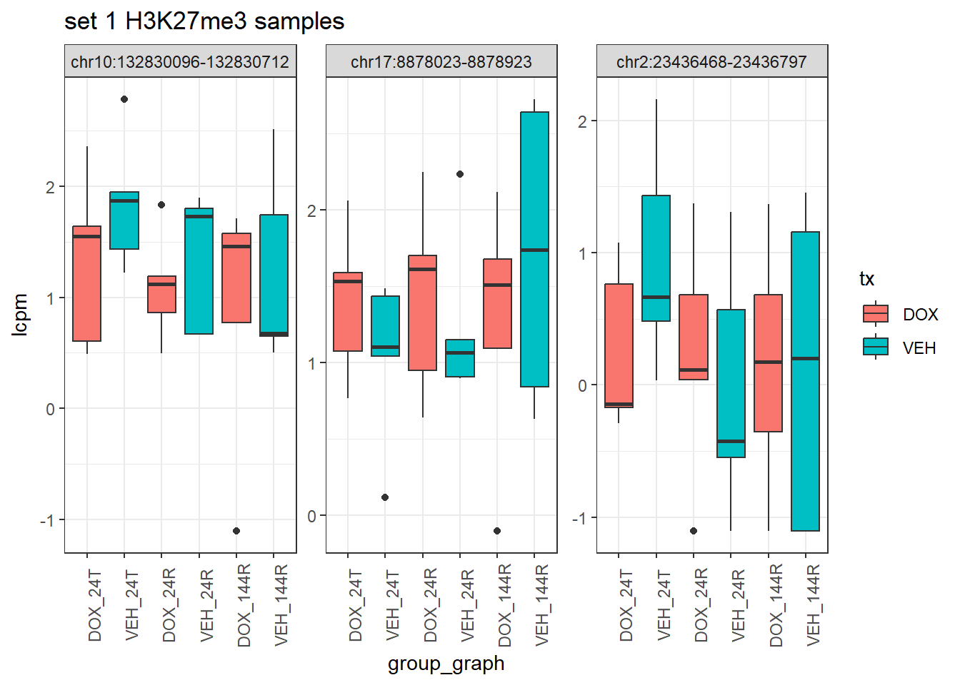
| Version | Author | Date |
|---|---|---|
| 1a7940a | reneeisnowhere | 2025-09-03 |
Set 2
H3K27me3_filt_lcpm %>%
  as.data.frame() %>%
  dplyr::filter(row.names(H3K27me3_filt_lcpm) %in% examp_H3K27me3_2) %>%
  ###pivot and add additional information from dataframe
  rownames_to_column("Peakid") %>%
  pivot_longer(., cols = !Peakid, names_to = "sample", values_to = "lcpm" ) %>%
  separate_wider_delim(., cols=sample, delim="_", names=c("ind","tx","time")) %>%
  mutate(ind=factor(ind, levels=c("Ind1", "Ind2", "Ind3", "Ind4","Ind5")),
         tx=factor(tx,levels = c("DOX","VEH")),
         time=factor(time, levels=c("24T","24R","144R")),
         group_graph= paste0(tx, "_", time),
         group=paste0("H3K27me3_",time),
      group_graph = factor(group_graph, levels = c(
        "DOX_24T",  "VEH_24T",
        "DOX_24R",  "VEH_24R",
        "DOX_144R",  "VEH_144R"))) %>%

  ggplot(., aes(x=group_graph, y=lcpm)) +
  geom_boxplot(aes(fill=tx))+
  facet_wrap(~Peakid, scales="free")+
  theme_bw()+
  theme(axis.text.x=element_text(angle = 90))+
  ggtitle("set 2 H3K27me3 samples")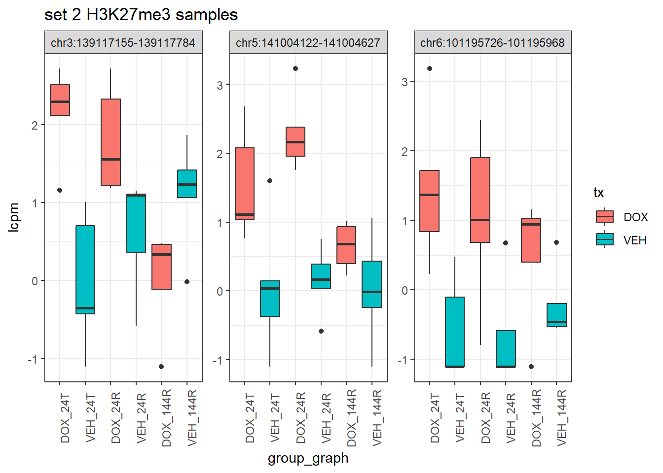
| Version | Author | Date |
|---|---|---|
| 1a7940a | reneeisnowhere | 2025-09-03 |
all_H3K27me3_regions_gr <- all_H3K27me3_regions %>%
    tidyr::separate(., col = "Peakid", into=c("seqnames","range"), sep = ":", remove=FALSE) %>%
  tidyr::separate(., col = "range", into=c("start","end"), sep = "-") %>%
  GRanges()

H3K27me3_set1_gr <- H3K27me3_set1 %>%
  tidyr::separate(., col = ".", into=c("seqnames","range"), sep = ":", remove=FALSE) %>%
  tidyr::separate(., col = "range", into=c("start","end"), sep = "-") %>%
  dplyr::rename("Peakid"=".") %>%
  GRanges()

H3K27me3_set2_gr <- H3K27me3_set2 %>%
  tidyr::separate(., col = ".", into=c("seqnames","range"), sep = ":", remove=FALSE) %>%
  tidyr::separate(., col = "range", into=c("start","end"), sep = "-") %>%
  dplyr::rename("Peakid"=".") %>%
  GRanges()


H3K27me3_list <- list("Set_1"=H3K27me3_set1_gr,"Set_2"=H3K27me3_set2_gr,"all_H3K27me3_regions"=all_H3K27me3_regions_gr)


# peakAnnoList_H3K27me3 <- lapply(H3K27me3_list, annotatePeak, tssRegion =c(-2000,2000), TxDb=txdb)
#
# saveRDS(peakAnnoList_H3K27me3, "data/motif_lists/H3K27me3_annotated_peaks.RDS")
peakAnnoList_H3K27me3 <- readRDS("data/motif_lists/H3K27me3_annotated_peaks.RDS")

plotAnnoBar(peakAnnoList_H3K27me3[c(3,1,2)])+
  ggtitle("H3K27me3 Feature Distribution")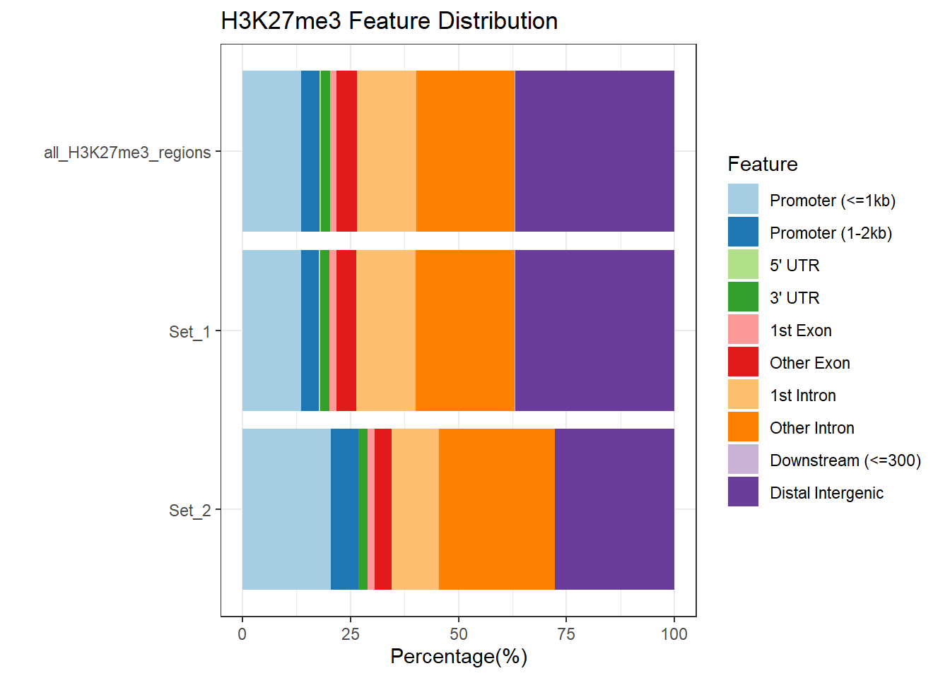
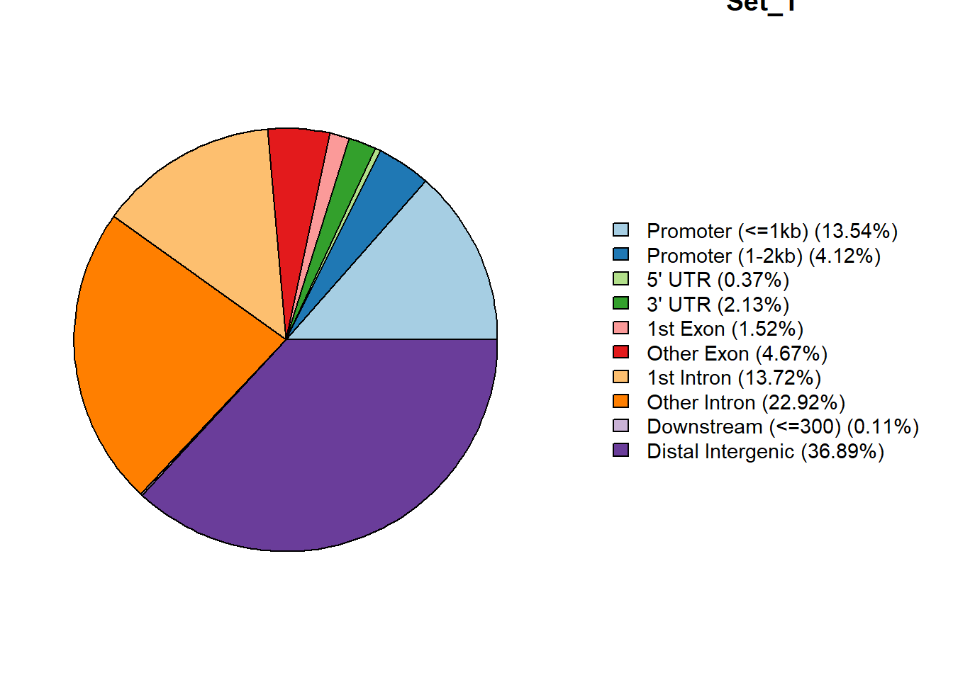
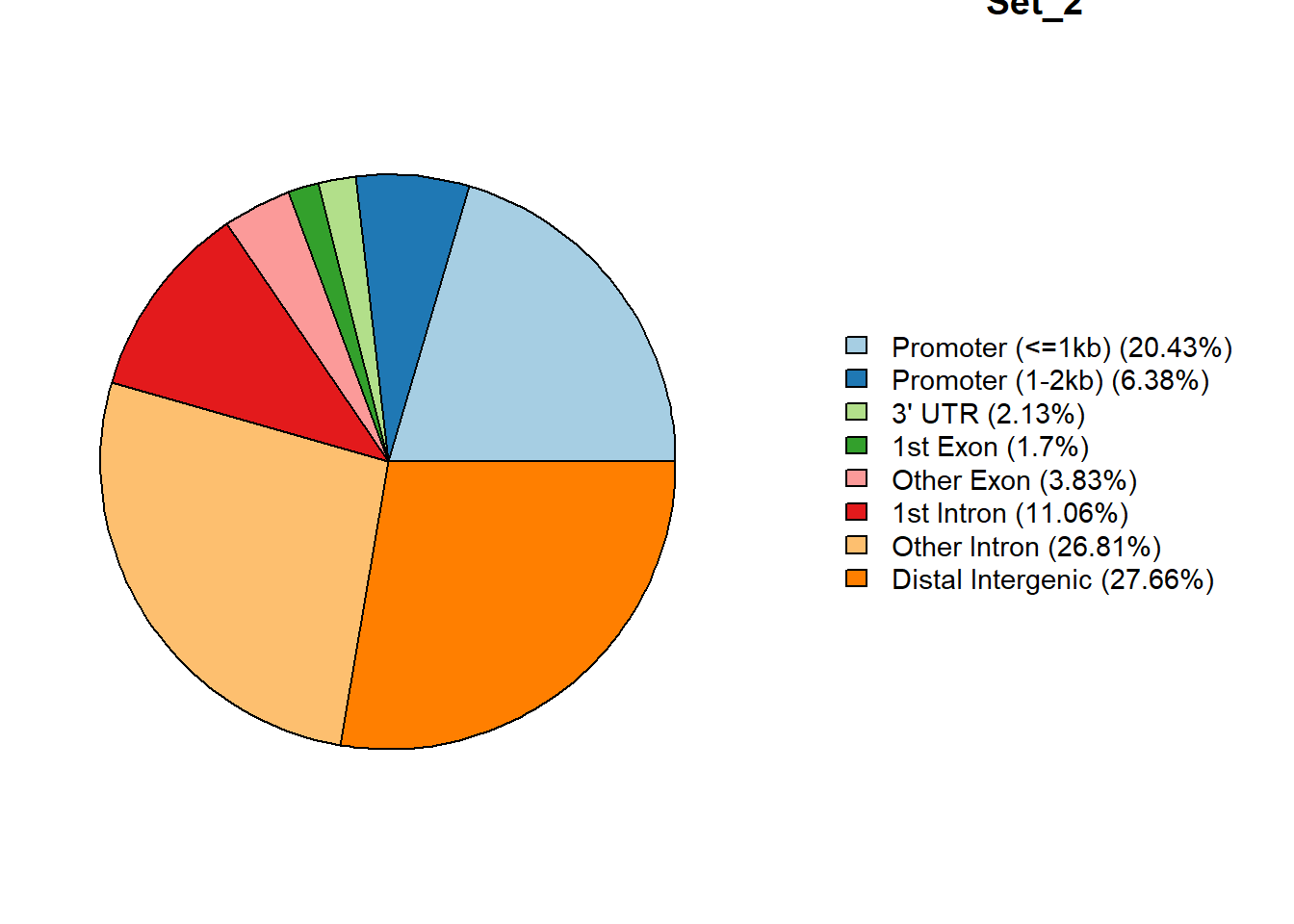
# pie_plots_H3K27me3 <-   map(peakAnnoList_H3K27me3, ~ plotAnnoPie(.x))
for(nm in names(peakAnnoList_H3K27me3)) {
  plotAnnoPie(peakAnnoList_H3K27me3[[nm]])
  title(main = nm)  # base R title
}
| Version | Author | Date |
|---|---|---|
| 1a7940a | reneeisnowhere | 2025-09-03 |
| Version | Author | Date |
|---|---|---|
| 1a7940a | reneeisnowhere | 2025-09-03 |

Histone proportions
H3K27me3_lookup <- imap_dfr(peakAnnoList_H3K27me3[1:2], ~
  tibble(Peakid = .x@anno$Peakid, cluster = .y))
all_H3K27me3_regions %>%
  mutate(group="H3K27me3") %>%
  left_join(., H3K27me3_lookup) %>%
   tidyr::replace_na(list(cluster = "NA")) %>%
  ggplot(., aes(y=group,fill=cluster))+
  geom_bar()+
  geom_text(aes( label = scales::percent(..prop..),
                   x= ..prop.. ), stat= "count", vjust = -.5)+
  ggtitle("H3K27me3 proportions of ROIs")+
  theme_classic()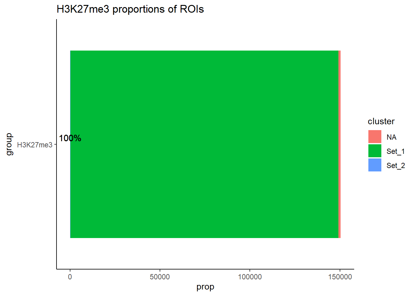
all_H3K27me3_regions %>%
  mutate(group="H3K27me3") %>%
  left_join(., H3K27me3_lookup) %>%
   tidyr::replace_na(list(cluster = "NA")) %>%
  mutate(cluster=factor(cluster, levels = c("Set_1","Set_2","NA"))) %>%
  ggplot(., aes(x=cluster,y = after_stat(prop),fill=cluster, group=1))+
  geom_bar(aes(stat="count"))+
  geom_text(aes( label = scales::percent(after_stat(prop))),
            stat= "count", vjust = -.5)+
  scale_y_continuous(
    labels = scales::percent,
    expand = expansion(mult = c(0, 0.1))
  ) +
  ggtitle("H3K27me3 proportions of ROIs")+
  theme_classic()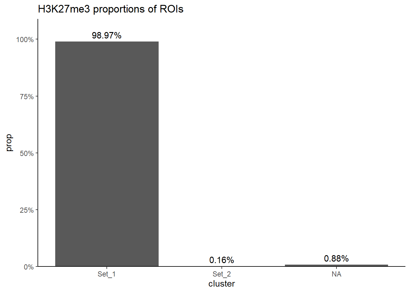
all_H3K27me3_regions %>%
  mutate(group="H3K27me3") %>%
  left_join(., H3K27me3_lookup) %>%
   tidyr::replace_na(list(cluster = "NA")) %>%
  group_by(cluster) %>%
  tally(name = "n_ROIs") %>%
  ungroup() %>%
  DT::datatable(
    rownames = FALSE,
    caption = htmltools::tags$caption(
      style = "caption-side: top; text-align: left;",
      "H3K27me3 ROI counts per cluster"
    ),
    options = list(
      pageLength = 10,
      autoWidth = TRUE,
      dom = "tip"
    )
  )
LFC H3K27me3
Set1
# H3K27me3_toptable_list %>%
#   dplyr::filter(genes %in% H3K27me3_set1$.) %>%
#   dplyr::select(group,genes,logFC) %>%
#   mutate(group=factor(group, levels = c("H3K27me3_24T","H3K27me3_24R","H3K27me3_144R"))) %>%
#   ggplot(., aes(x=group, y=logFC))+
#   geom_boxplot(aes(fill=group))+
#   geom_signif(comparisons = list(c("H3K27me3_24T", "H3K27me3_144R"),
#                                  c("H3K27me3_24T","H3K27me3_24R"),
#                                  c("H3K27me3_24R", "H3K27me3_144R")),
#                               step_increase = 0.1,
#               map_signif_level = FALSE,
#               test = "wilcox.test")+
#   theme_bw()+
#   ggtitle("LFC across time for H3K27me3 set1")


H3K27me3_toptable_list %>%
  dplyr::filter(genes %in% H3K27me3_set1$.) %>%
  dplyr::select(group,genes,logFC) %>%
  mutate(group=factor(group, levels = c("H3K27me3_24T","H3K27me3_24R","H3K27me3_144R")),
         logFC=abs(logFC)) %>%
  ggplot(., aes(x=group, y=logFC))+
  geom_boxplot(aes(fill=group))+
  geom_signif(comparisons = list(c("H3K27me3_24T", "H3K27me3_144R"),
                                 c("H3K27me3_24T","H3K27me3_24R"),
                                 c("H3K27me3_24R", "H3K27me3_144R")),
                              step_increase = 0.1,
              map_signif_level = FALSE,
              test = "wilcox.test")+
  theme_bw()+
  ggtitle("Absolute LFC across time for H3K27me3 set1")
| Version | Author | Date |
|---|---|---|
| 1a7940a | reneeisnowhere | 2025-09-03 |
  set1_27me3 <- H3K27me3_toptable_list %>%
  dplyr::filter(genes %in% H3K27me3_set1$.) %>%
   dplyr::select(group,genes,logFC) %>%
   mutate(group=factor(group, levels = c("H3K27me3_24T","H3K27me3_24R","H3K27me3_144R")),
         logFC=abs(logFC)) %>%
  group_by(group) %>%
  summarize(med_Set1=median(logFC),.groups="drop")
set2
# H3K27me3_toptable_list %>%
#   dplyr::filter(genes %in% H3K27me3_set2$.) %>%
#   dplyr::select(group,genes,logFC) %>%
#   mutate(group=factor(group, levels = c("H3K27me3_24T","H3K27me3_24R","H3K27me3_144R"))) %>%
#   ggplot(., aes(x=group, y=logFC))+
#   geom_boxplot(aes(fill=group))+
#   geom_signif(comparisons = list(c("H3K27me3_24T", "H3K27me3_144R"),
#                                  c("H3K27me3_24T","H3K27me3_24R"),
#                                  c("H3K27me3_24R", "H3K27me3_144R")),
#                               step_increase = 0.1,
#               map_signif_level = FALSE,
#               test = "wilcox.test")+
#   theme_bw()+
#   ggtitle("LFC across time for H3K27me3 set2")


H3K27me3_toptable_list %>%
  dplyr::filter(genes %in% H3K27me3_set2$.) %>%
  dplyr::select(group,genes,logFC) %>%
  mutate(group=factor(group, levels = c("H3K27me3_24T","H3K27me3_24R","H3K27me3_144R")),
         logFC=abs(logFC)) %>%
  ggplot(., aes(x=group, y=logFC))+
  geom_boxplot(aes(fill=group))+
  geom_signif(comparisons = list(c("H3K27me3_24T", "H3K27me3_144R"),
                                 c("H3K27me3_24T","H3K27me3_24R"),
                                 c("H3K27me3_24R", "H3K27me3_144R")),
                              step_increase = 0.1,
              map_signif_level = FALSE,
              test = "wilcox.test")+
  theme_bw()+
  ggtitle("Absolute LFC across time for H3K27me3 set2")
| Version | Author | Date |
|---|---|---|
| 1a7940a | reneeisnowhere | 2025-09-03 |
  H3K27me3_toptable_list %>%
  dplyr::filter(genes %in% H3K27me3_set2$.) %>%
  dplyr::select(group,genes,logFC) %>%
   mutate(group=factor(group, levels = c("H3K27me3_24T","H3K27me3_24R","H3K27me3_144R")),
         logFC=abs(logFC)) %>%
  group_by(group) %>%
  summarize(med_Set2=median(logFC),.groups="drop") %>%
  left_join(set1_27me3,by = "group") %>%
  pivot_longer(cols=!group, values_to = "median_LFC", names_to = "set") %>%
  ggplot(., aes(x=group, y=median_LFC, group=set, color=set))+
  geom_point()+
  geom_line(aes(alpha = 0.8))+
  theme_bw()+
  ggtitle("LFC across time for H3K27me3 sets")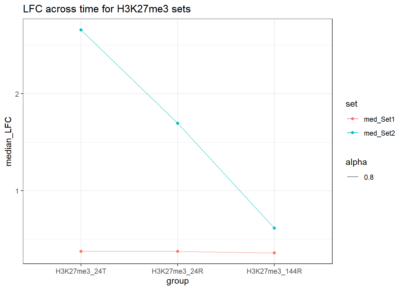
Top 100
This is the calculation of Top 100 in each category, then united
cormotif_initial_H3K27me3 <- readRDS("data/Cormotif_data/Cormotif_initial_H3K27me3.RDS")
row.names(cormotif_initial_H3K27me3$bestmotif$clustlike) <- row.names(H3K27me3_filt_lcpm)
H3K27me3_clustlike <- cormotif_initial_H3K27me3$bestmotif$clustlike %>%
  as.data.frame() %>%
  rownames_to_column("Peakid")

H3K27me3_clusters <- list(
  Set1="V1",
  Set2="V2")


Sets_H3K27me3 <- H3K27me3_toptable_list %>%
  mutate(cluster=case_when(genes %in% H3K27me3_set1$. ~ "Set1",
                           genes %in% H3K27me3_set2$. ~ "Set2",
                           TRUE ~ "not_assigned")) %>%
  left_join(., H3K27me3_clustlike,by=c("genes"="Peakid")) %>%
  dplyr::filter(cluster!="not_assigned")

###This code uses the H3K27me3_clusters list and filters through Sets_H3K27me3 data frame by selecting
Sets_H3K27me3_top <- map_dfr(names(H3K27me3_clusters), function(cl) {
  col <- H3K27me3_clusters[[cl]]
  Sets_H3K27me3 %>%
    filter(cluster == cl) %>%
    # group_by(group) %>%
    slice_max(order_by = .data[[col]], n = 100)
}) %>%
  ungroup()

## now plot

Sets_H3K27me3_top %>%
  mutate(group=factor(group, levels = c("H3K27me3_24T","H3K27me3_24R","H3K27me3_144R")),
         cluster=factor(cluster, levels=c("Set1","Set2"))) %>%
  ggplot(., aes(x= group,y = logFC, group = interaction(cluster, genes), color=cluster))+
  geom_point()+
  geom_line(aes(alpha = 0.8))+
  theme_bw()+
  facet_wrap(~cluster)+
  ggtitle("LFC across time for H3K27me3 top 100 by Set")+
  theme(axis.text.x = element_text(angle=90) )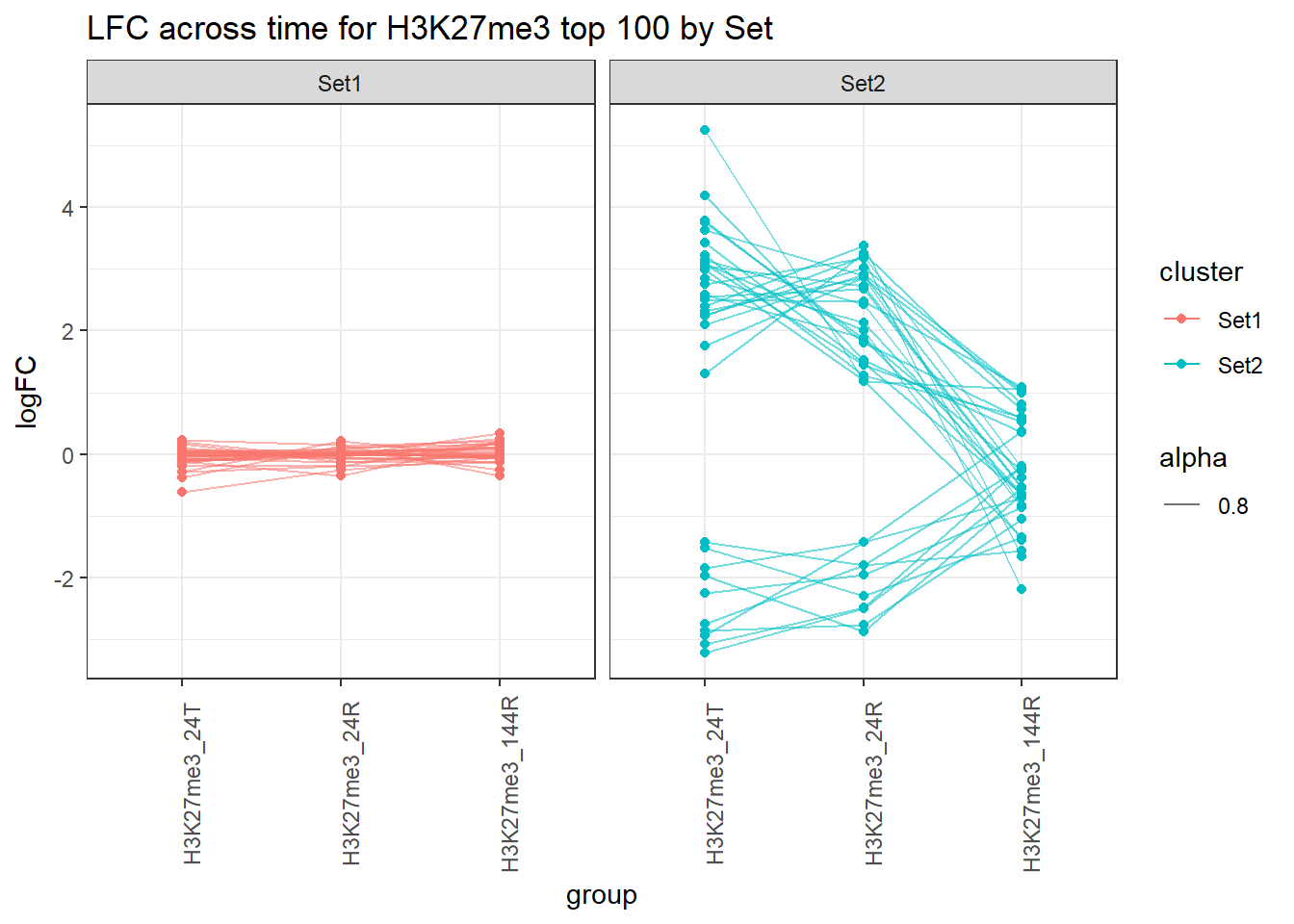
| Version | Author | Date |
|---|---|---|
| 1ce5e71 | reneeisnowhere | 2025-09-16 |
# saveRDS(Sets_H3K27me3_top,"data/motif_lists/H3K27me3_toplistbymotif.RDS")H3K36me3 motifs samples
Set 1
# slice_sample(H3K36me3_set1,n = 3, replace=FALSE)
examp_H3K36me3_1 <-#slice_sample(H3K36me3_set1,n = 3, replace=FALSE)
  c("chr6:106975625-106975872","chr17:17259340-17260414","chr14:91506581-91506995")
examp_H3K36me3_2 <-#slice_sample(H3K36me3_set2,n = 3, replace=FALSE)
  # c("chr2:191013033-191013351","chr5:66597066-66597500","chr16:22232346-22233214")
c("chr17:3656403-3665271","chr6:118573949-118574870","chr1:164799555-164800172")


H3K36me3_filt_lcpm %>%
  as.data.frame() %>%
  dplyr::filter(row.names(H3K36me3_filt_lcpm) %in% examp_H3K36me3_1) %>%
  ###pivot and add additional information from dataframe
  rownames_to_column("Peakid") %>%
  pivot_longer(., cols = !Peakid, names_to = "sample", values_to = "lcpm" ) %>%
  separate_wider_delim(., cols=sample, delim="_", names=c("ind","tx","time")) %>%
  mutate(ind=factor(ind, levels=c("Ind1", "Ind2", "Ind3", "Ind4","Ind5")),
         tx=factor(tx,levels = c("DOX","VEH")),
         time=factor(time, levels=c("24T","24R","144R")),
         group_graph= paste0(tx, "_", time),
         group=paste0("H3K36me3_",time),
      group_graph = factor(group_graph, levels = c(
        "DOX_24T",  "VEH_24T",
        "DOX_24R",  "VEH_24R",
        "DOX_144R",  "VEH_144R"))) %>%

  ggplot(., aes(x=group_graph, y=lcpm)) +
  geom_boxplot(aes(fill=tx))+
  facet_wrap(~Peakid, scales="free")+
  theme_bw()+
  theme(axis.text.x=element_text(angle = 90))+
  ggtitle("set 1 H3K36me3 samples")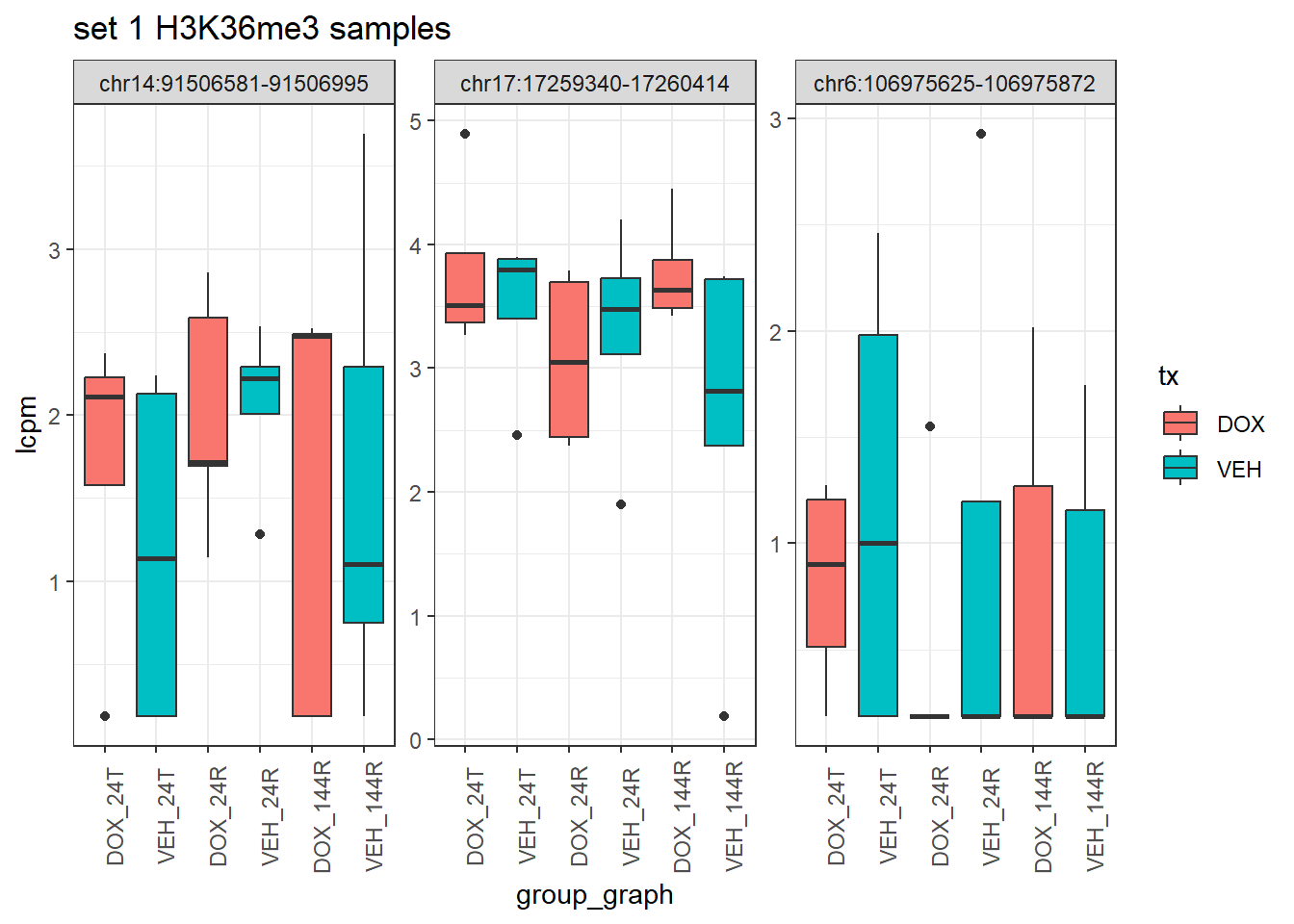
| Version | Author | Date |
|---|---|---|
| 1a7940a | reneeisnowhere | 2025-09-03 |
Set 2
H3K36me3_filt_lcpm %>%
  as.data.frame() %>%
  dplyr::filter(row.names(H3K36me3_filt_lcpm) %in% examp_H3K36me3_2) %>%
  ###pivot and add additional information from dataframe
  rownames_to_column("Peakid") %>%
  pivot_longer(., cols = !Peakid, names_to = "sample", values_to = "lcpm" ) %>%
  separate_wider_delim(., cols=sample, delim="_", names=c("ind","tx","time")) %>%
  mutate(ind=factor(ind, levels=c("Ind1", "Ind2", "Ind3", "Ind4","Ind5")),
         tx=factor(tx,levels = c("DOX","VEH")),
         time=factor(time, levels=c("24T","24R","144R")),
         group_graph= paste0(tx, "_", time),
         group=paste0("H3K36me3_",time),
      group_graph = factor(group_graph, levels = c(
        "DOX_24T",  "VEH_24T",
        "DOX_24R",  "VEH_24R",
        "DOX_144R",  "VEH_144R"))) %>%

  ggplot(., aes(x=group_graph, y=lcpm)) +
  geom_boxplot(aes(fill=tx))+
  facet_wrap(~Peakid, scales="free")+
  theme_bw()+
  theme(axis.text.x=element_text(angle = 90))+
  ggtitle("set 2 H3K36me3 samples")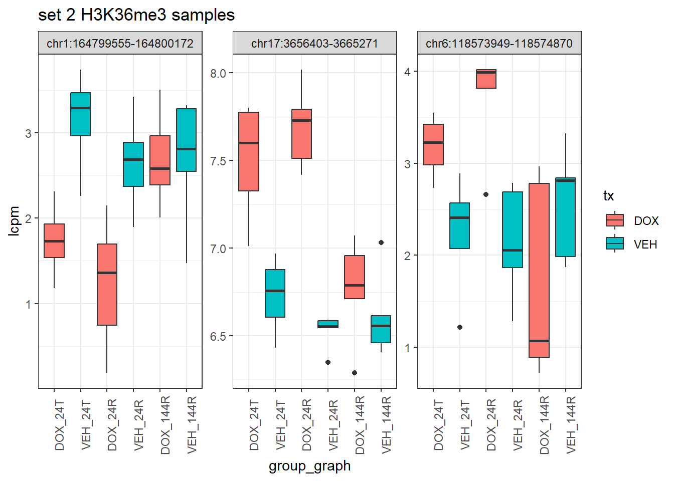
| Version | Author | Date |
|---|---|---|
| 1a7940a | reneeisnowhere | 2025-09-03 |
all_H3K36me3_regions_gr <- all_H3K36me3_regions %>%
    tidyr::separate(., col = "Peakid", into=c("seqnames","range"), sep = ":", remove=FALSE) %>%
  tidyr::separate(., col = "range", into=c("start","end"), sep = "-") %>%
  GRanges()

H3K36me3_set1_gr <- H3K36me3_set1 %>%
  tidyr::separate(., col = ".", into=c("seqnames","range"), sep = ":", remove=FALSE) %>%
  tidyr::separate(., col = "range", into=c("start","end"), sep = "-") %>%
  dplyr::rename("Peakid"=".") %>%
  GRanges()

H3K36me3_set2_gr <- H3K36me3_set2 %>%
  tidyr::separate(., col = ".", into=c("seqnames","range"), sep = ":", remove=FALSE) %>%
  tidyr::separate(., col = "range", into=c("start","end"), sep = "-") %>%
  dplyr::rename("Peakid"=".") %>%
  GRanges()


H3K36me3_list <- list("Set_1"=H3K36me3_set1_gr,"Set_2"=H3K36me3_set2_gr, "all_H3K36me3_regions"=all_H3K36me3_regions_gr)


# peakAnnoList_H3K36me3 <- lapply(H3K36me3_list, annotatePeak, tssRegion =c(-2000,2000), TxDb=txdb)
# #
# saveRDS(peakAnnoList_H3K36me3, "data/motif_lists/H3K36me3_annotated_peaks.RDS")
peakAnnoList_H3K36me3 <- readRDS("data/motif_lists/H3K36me3_annotated_peaks.RDS")

plotAnnoBar(peakAnnoList_H3K36me3[c(3,1,2)])+
  ggtitle("H3K36me3 Feature Distribution")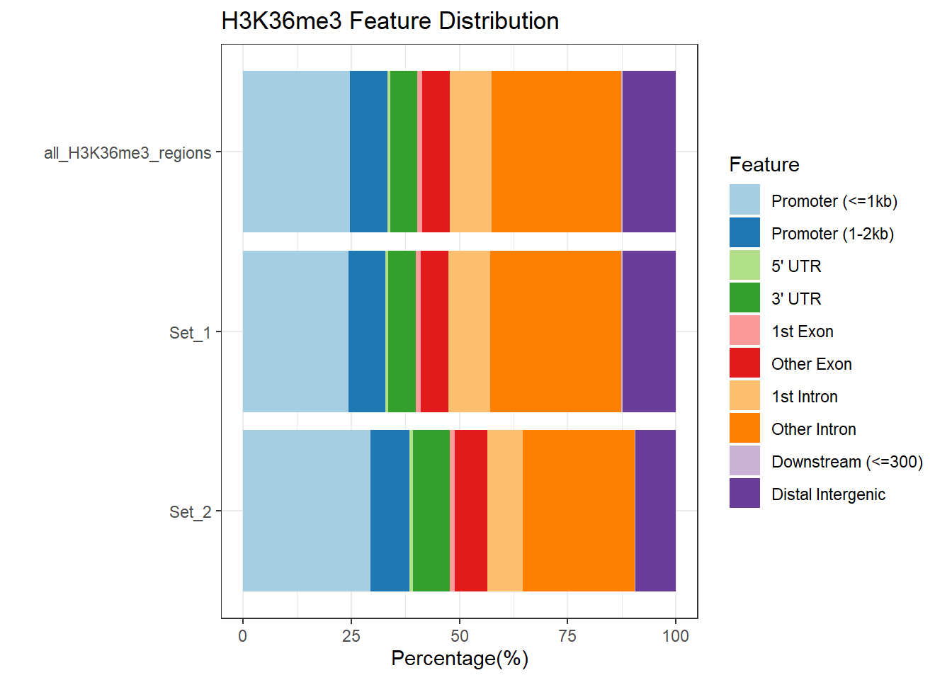
| Version | Author | Date |
|---|---|---|
| 1a7940a | reneeisnowhere | 2025-09-03 |
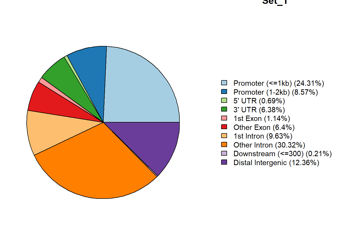
# pie_plots_H3K36me3 <-   map(peakAnnoList_H3K36me3, ~ plotAnnoPie(.x))
for(nm in names(peakAnnoList_H3K36me3)) {
  plotAnnoPie(peakAnnoList_H3K36me3[[nm]])
  title(main = nm)  # base R title
}
| Version | Author | Date |
|---|---|---|
| 1a7940a | reneeisnowhere | 2025-09-03 |

| Version | Author | Date |
|---|---|---|
| 1a7940a | reneeisnowhere | 2025-09-03 |

| Version | Author | Date |
|---|---|---|
| 1a7940a | reneeisnowhere | 2025-09-03 |
Histone proportions
H3K36me3_lookup <- imap_dfr(peakAnnoList_H3K36me3[1:2], ~
  tibble(Peakid = .x@anno$Peakid, cluster = .y))
all_H3K36me3_regions %>%
  mutate(group="H3K36me3") %>%
  left_join(., H3K36me3_lookup) %>%
   tidyr::replace_na(list(cluster = "NA")) %>%
  ggplot(., aes(y=group,fill=cluster))+
  geom_bar()+
  geom_text(aes( label = scales::percent(..prop..),
                   x= ..prop.. ), stat= "count", vjust = -.5)+
  ggtitle("H3K36me3 proportions of ROIs")+
  theme_classic()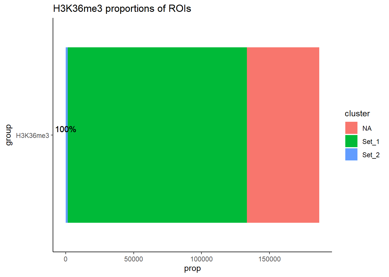
all_H3K36me3_regions %>%
  mutate(group="H3K36me3") %>%
  left_join(., H3K36me3_lookup) %>%
   tidyr::replace_na(list(cluster = "NA")) %>%
  mutate(cluster=factor(cluster, levels = c("Set_1","Set_2","NA"))) %>%
  ggplot(., aes(x=cluster,y = after_stat(prop), group=1))+
  geom_bar(aes(stat="count"))+
  geom_text(aes( label = scales::percent(after_stat(prop))),
            stat= "count", vjust = -.5)+
  scale_y_continuous(
    labels = scales::percent,
    expand = expansion(mult = c(0, 0.1))
  ) +
  ggtitle("H3K36me3 proportions of ROIs")+
  theme_classic()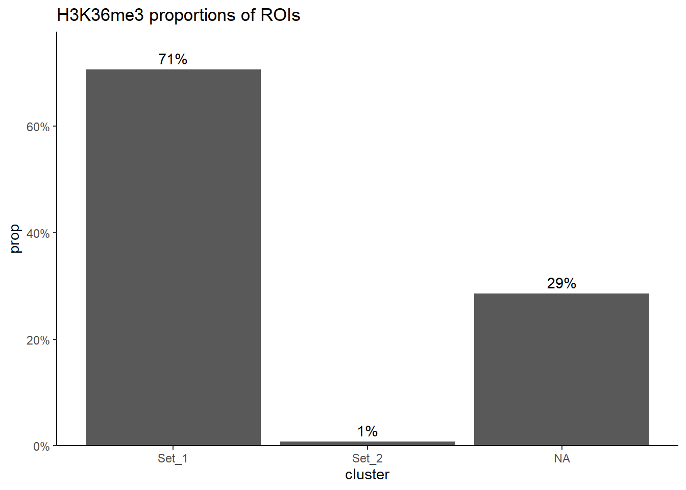
all_H3K36me3_regions %>%
  mutate(group="H3K36me3") %>%
  left_join(., H3K36me3_lookup) %>%
   tidyr::replace_na(list(cluster = "NA")) %>%
  group_by(cluster) %>%
  tally(name = "n_ROIs") %>%
  ungroup() %>%
  DT::datatable(
    rownames = FALSE,
    caption = htmltools::tags$caption(
      style = "caption-side: top; text-align: left;",
      "H3K36me3 ROI counts per cluster"
    ),
    options = list(
      pageLength = 10,
      autoWidth = TRUE,
      dom = "tip",
      columnDefs = list(
        list(className = "dt-head-center", targets = "_all"),
        list(className = "dt-center", targets = "_all")
      )
  ))
LFC H3K36me3
Set1
# H3K36me3_toptable_list %>%
#   dplyr::filter(genes %in% H3K36me3_set1$.) %>%
#   dplyr::select(group,genes,logFC) %>%
#   mutate(group=factor(group, levels = c("H3K36me3_24T","H3K36me3_24R","H3K36me3_144R"))) %>%
#   ggplot(., aes(x=group, y=logFC))+
#   geom_boxplot(aes(fill=group))+
#   geom_signif(comparisons = list(c("H3K36me3_24T", "H3K36me3_144R"),
#                                  c("H3K36me3_24T","H3K36me3_24R"),
#                                  c("H3K36me3_24R", "H3K36me3_144R")),
#                               step_increase = 0.1,
#               map_signif_level = FALSE,
#               test = "wilcox.test")+
#   theme_bw()+
#   ggtitle("LFC across time for H3K36me3 set1")


H3K36me3_toptable_list %>%
  dplyr::filter(genes %in% H3K36me3_set1$.) %>%
  dplyr::select(group,genes,logFC) %>%
  mutate(group=factor(group, levels = c("H3K36me3_24T","H3K36me3_24R","H3K36me3_144R")),
         logFC=abs(logFC)) %>%
  ggplot(., aes(x=group, y=logFC))+
  geom_boxplot(aes(fill=group))+
  geom_signif(comparisons = list(c("H3K36me3_24T", "H3K36me3_144R"),
                                 c("H3K36me3_24T","H3K36me3_24R"),
                                 c("H3K36me3_24R", "H3K36me3_144R")),
                              step_increase = 0.1,
              map_signif_level = FALSE,
              test = "wilcox.test")+
  theme_bw()+
  ggtitle("Absolute LFC across time for H3K36me3 set1")
| Version | Author | Date |
|---|---|---|
| 1a7940a | reneeisnowhere | 2025-09-03 |
 set1_36me3 <- H3K36me3_toptable_list %>%
  dplyr::filter(genes %in% H3K36me3_set1$.) %>%
  dplyr::select(group,genes,logFC) %>%
   mutate(group=factor(group, levels = c("H3K36me3_24T","H3K36me3_24R","H3K36me3_144R")),
         logFC=abs(logFC)) %>%
  group_by(group) %>%
  summarize(med_Set1=median(logFC),.groups="drop")
set2
#
# H3K36me3_toptable_list %>%
#   dplyr::filter(genes %in% H3K36me3_set2$.) %>%
#   dplyr::select(group,genes,logFC) %>%
#   mutate(group=factor(group, levels = c("H3K36me3_24T","H3K36me3_24R","H3K36me3_144R"))) %>%
#   ggplot(., aes(x=group, y=logFC))+
#   geom_boxplot(aes(fill=group))+
#   geom_signif(comparisons = list(c("H3K36me3_24T", "H3K36me3_144R"),
#                                  c("H3K36me3_24T","H3K36me3_24R"),
#                                  c("H3K36me3_24R", "H3K36me3_144R")),
#                               step_increase = 0.1,
#               map_signif_level = FALSE,
#               test = "wilcox.test")+
#   theme_bw()+
#   ggtitle("LFC across time for H3K36me3 set2")


H3K36me3_toptable_list %>%
  dplyr::filter(genes %in% H3K36me3_set2$.) %>%
  dplyr::select(group,genes,logFC) %>%
  mutate(group=factor(group, levels = c("H3K36me3_24T","H3K36me3_24R","H3K36me3_144R")),
         logFC=abs(logFC)) %>%
  ggplot(., aes(x=group, y=logFC))+
  geom_boxplot(aes(fill=group))+
  geom_signif(comparisons = list(c("H3K36me3_24T", "H3K36me3_144R"),
                                 c("H3K36me3_24T","H3K36me3_24R"),
                                 c("H3K36me3_24R", "H3K36me3_144R")),
                              step_increase = 0.1,
              map_signif_level = FALSE,
              test = "wilcox.test")+
  theme_bw()+
  ggtitle("Absolute LFC across time for H3K36me3 set2")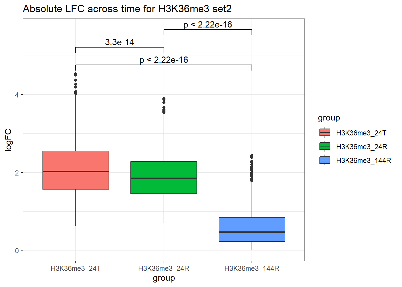
| Version | Author | Date |
|---|---|---|
| 1a7940a | reneeisnowhere | 2025-09-03 |
 H3K36me3_toptable_list %>%
  dplyr::filter(genes %in% H3K36me3_set2$.) %>%
  dplyr::select(group,genes,logFC) %>%
   mutate(group=factor(group, levels = c("H3K36me3_24T","H3K36me3_24R","H3K36me3_144R")),
         logFC=abs(logFC)) %>%
  group_by(group) %>%
  summarize(med_Set2=median(logFC),.groups="drop") %>%
  left_join(set1_36me3,by = "group") %>%
  pivot_longer(cols=!group, values_to = "median_LFC", names_to = "set") %>%
  ggplot(., aes(x=group, y=median_LFC, group=set, color=set))+
  geom_point()+
  geom_line(aes(alpha = 0.8))+
  theme_bw()+
  ggtitle("LFC across time for H3K36me3 sets")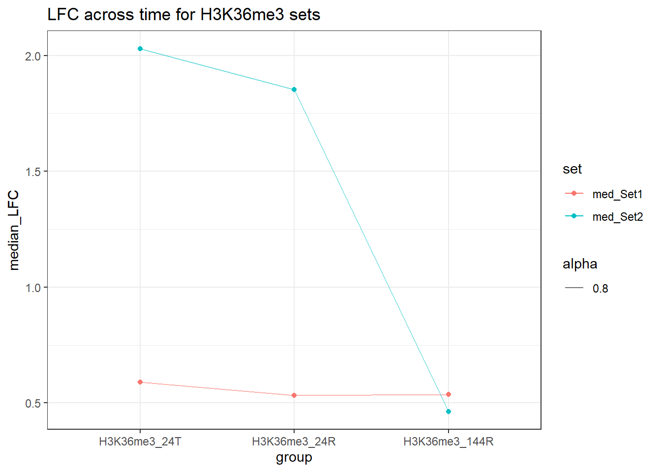
Top 100
This is the calculation of Top 100 in each category, then united
cormotif_initial_H3K36me3 <- readRDS("data/Cormotif_data/Cormotif_initial_H3K36me3.RDS")
row.names(cormotif_initial_H3K36me3$bestmotif$clustlike) <- row.names(H3K36me3_filt_lcpm)
H3K36me3_clustlike <- cormotif_initial_H3K36me3$bestmotif$clustlike %>%
  as.data.frame() %>%
  rownames_to_column("Peakid")

H3K36me3_clusters <- list(
  Set1="V1",
  Set2="V2")


Sets_H3K36me3 <- H3K36me3_toptable_list %>%
  mutate(cluster=case_when(genes %in% H3K36me3_set1$. ~ "Set1",
                           genes %in% H3K36me3_set2$. ~ "Set2",
                           TRUE ~ "not_assigned")) %>%
  left_join(., H3K36me3_clustlike,by=c("genes"="Peakid")) %>%
  dplyr::filter(cluster!="not_assigned")

###This code uses the H3K36me3_clusters list and filters through Sets_H3K36me3 data frame by selecting
Sets_H3K36me3_top <- map_dfr(names(H3K36me3_clusters), function(cl) {
  col <- H3K36me3_clusters[[cl]]
  Sets_H3K36me3 %>%
    filter(cluster == cl) %>%
    # group_by(group) %>%
    slice_max(order_by = .data[[col]], n = 100)
}) %>%
  ungroup()

## now plot

Sets_H3K36me3_top %>%
  mutate(group=factor(group, levels = c("H3K36me3_24T","H3K36me3_24R","H3K36me3_144R")),
         cluster=factor(cluster, levels=c("Set1","Set2"))) %>%
  ggplot(., aes(x= group,y = logFC, group = interaction(cluster, genes), color=cluster))+
  geom_point()+
  geom_line(aes(alpha = 0.8))+
  theme_bw()+
  facet_wrap(~cluster)+
  ggtitle("LFC across time for H3K36me3 top 100 by Set")+
  theme(axis.text.x = element_text(angle=90) )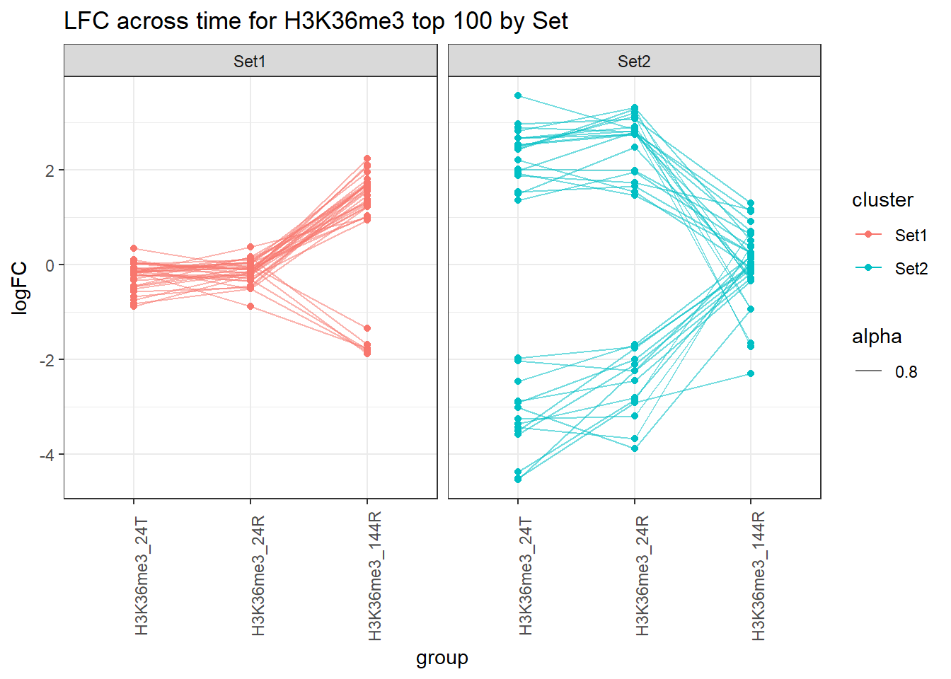
| Version | Author | Date |
|---|---|---|
| 1ce5e71 | reneeisnowhere | 2025-09-16 |
# saveRDS(Sets_H3K36me3_top,"data/motif_lists/H3K36me3_toplistbymotif.RDS")H3K9me3 motifs samples
Set 1
# slice_sample(H3K9me3_set3,n = 3, replace=FALSE)
examp_H3K9me3_1 <-#slice_sample(H3K9me3_set1,n = 3, replace=FALSE)
  c("chr7:101406339-101407813","chr6:147512995-147514238","chr10:66432792-66433011")
examp_H3K9me3_2 <-#slice_sample(H3K9me3_set2,n = 3, replace=FALSE)
  c("chr2:120985518-120985865" ,   "chr7:926998-927207","chr12:108895126-108895841")

examp_H3K9me3_3 <- #slice_sample(H3K9me3_set3,n = 3, replace=FALSE)
  c("chr6:44276324-44278629","chr7:906806-907939"  ,"chr20:63682374-63682947")


H3K9me3_filt_lcpm %>%
  as.data.frame() %>%
  dplyr::filter(row.names(H3K9me3_filt_lcpm) %in% examp_H3K9me3_1) %>%
  ###pivot and add additional information from dataframe
  rownames_to_column("Peakid") %>%
  pivot_longer(., cols = !Peakid, names_to = "sample", values_to = "lcpm" ) %>%
  separate_wider_delim(., cols=sample, delim="_", names=c("ind","tx","time")) %>%
  mutate(ind=factor(ind, levels=c("Ind1", "Ind2", "Ind3", "Ind4","Ind5")),
         tx=factor(tx,levels = c("DOX","VEH")),
         time=factor(time, levels=c("24T","24R","144R")),
         group_graph= paste0(tx, "_", time),
         group=paste0("H3K9me3_",time),
      group_graph = factor(group_graph, levels = c(
        "DOX_24T",  "VEH_24T",
        "DOX_24R",  "VEH_24R",
        "DOX_144R",  "VEH_144R"))) %>%

  ggplot(., aes(x=group_graph, y=lcpm)) +
  geom_boxplot(aes(fill=tx))+
  facet_wrap(~Peakid, scales="free")+
  theme_bw()+
  theme(axis.text.x=element_text(angle = 90))+
  ggtitle("set 1 H3K9me3 samples")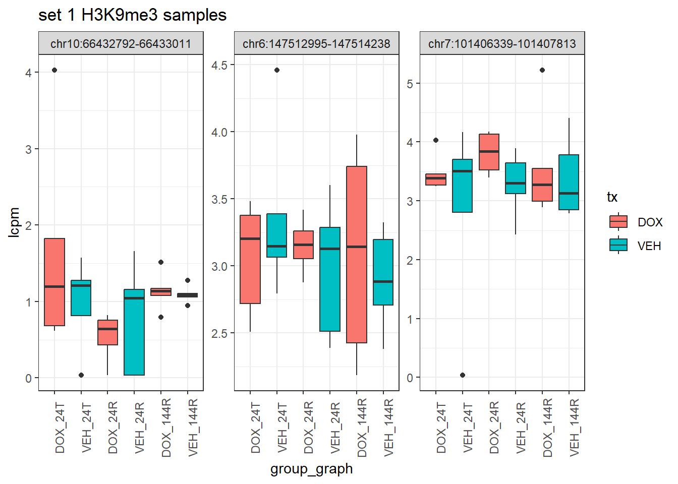
| Version | Author | Date |
|---|---|---|
| 1a7940a | reneeisnowhere | 2025-09-03 |
Set 2
H3K9me3_filt_lcpm %>%
  as.data.frame() %>%
  dplyr::filter(row.names(H3K9me3_filt_lcpm) %in% examp_H3K9me3_2) %>%
  ###pivot and add additional information from dataframe
  rownames_to_column("Peakid") %>%
  pivot_longer(., cols = !Peakid, names_to = "sample", values_to = "lcpm" ) %>%
  separate_wider_delim(., cols=sample, delim="_", names=c("ind","tx","time")) %>%
  mutate(ind=factor(ind, levels=c("Ind1", "Ind2", "Ind3", "Ind4","Ind5")),
         tx=factor(tx,levels = c("DOX","VEH")),
         time=factor(time, levels=c("24T","24R","144R")),
         group_graph= paste0(tx, "_", time),
         group=paste0("H3K9me3_",time),
      group_graph = factor(group_graph, levels = c(
        "DOX_24T",  "VEH_24T",
        "DOX_24R",  "VEH_24R",
        "DOX_144R",  "VEH_144R"))) %>%

  ggplot(., aes(x=group_graph, y=lcpm)) +
  geom_boxplot(aes(fill=tx))+
  facet_wrap(~Peakid, scales="free")+
  theme_bw()+
  theme(axis.text.x=element_text(angle = 90))+
  ggtitle("set 2 H3K9me3 samples")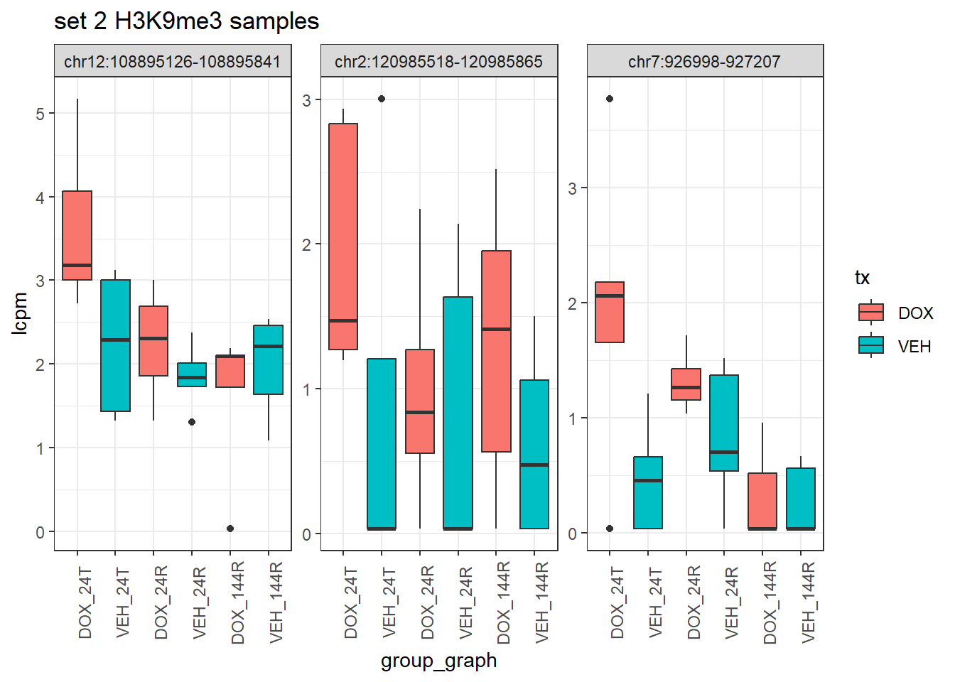
| Version | Author | Date |
|---|---|---|
| 1a7940a | reneeisnowhere | 2025-09-03 |
Set 3
H3K9me3_filt_lcpm %>%
  as.data.frame() %>%
  dplyr::filter(row.names(H3K9me3_filt_lcpm) %in% examp_H3K9me3_3) %>%
  ###pivot and add additional information from dataframe
  rownames_to_column("Peakid") %>%
  pivot_longer(., cols = !Peakid, names_to = "sample", values_to = "lcpm" ) %>%
  separate_wider_delim(., cols=sample, delim="_", names=c("ind","tx","time")) %>%
  mutate(ind=factor(ind, levels=c("Ind1", "Ind2", "Ind3", "Ind4","Ind5")),
         tx=factor(tx,levels = c("DOX","VEH")),
         time=factor(time, levels=c("24T","24R","144R")),
         group_graph= paste0(tx, "_", time),
         group=paste0("H3K9me3_",time),
      group_graph = factor(group_graph, levels = c(
        "DOX_24T",  "VEH_24T",
        "DOX_24R",  "VEH_24R",
        "DOX_144R",  "VEH_144R"))) %>%

  ggplot(., aes(x=group_graph, y=lcpm)) +
  geom_boxplot(aes(fill=tx))+
  facet_wrap(~Peakid, scales="free")+
  theme_bw()+
  theme(axis.text.x=element_text(angle = 90))+
  ggtitle("set 3 H3K9me3 samples")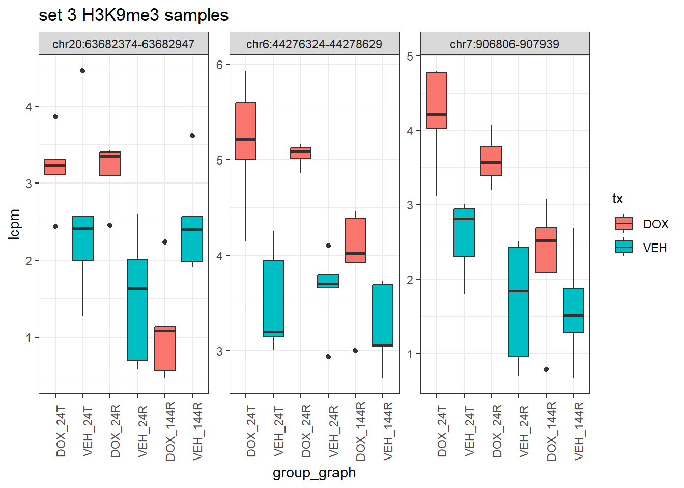
| Version | Author | Date |
|---|---|---|
| 1a7940a | reneeisnowhere | 2025-09-03 |
all_H3K9me3_regions_gr <- all_H3K9me3_regions %>%
    tidyr::separate(., col = "Peakid", into=c("seqnames","range"), sep = ":", remove=FALSE) %>%
  tidyr::separate(., col = "range", into=c("start","end"), sep = "-") %>%
  GRanges()


H3K9me3_set1_gr <- H3K9me3_set1 %>%
  tidyr::separate(., col = ".", into=c("seqnames","range"), sep = ":", remove=FALSE) %>%
  tidyr::separate(., col = "range", into=c("start","end"), sep = "-") %>%
  dplyr::rename("Peakid"=".") %>%
  GRanges()

H3K9me3_set2_gr <- H3K9me3_set2 %>%
  tidyr::separate(., col = ".", into=c("seqnames","range"), sep = ":", remove=FALSE) %>%
  tidyr::separate(., col = "range", into=c("start","end"), sep = "-") %>%
  dplyr::rename("Peakid"=".") %>%
  GRanges()

H3K9me3_set3_gr <- H3K9me3_set3 %>%
  tidyr::separate(., col = ".", into=c("seqnames","range"), sep = ":", remove=FALSE) %>%
  tidyr::separate(., col = "range", into=c("start","end"), sep = "-") %>%
  dplyr::rename("Peakid"=".") %>%
  GRanges()
H3K9me3_list <- list("Set_1"=H3K9me3_set1_gr,"Set_2"=H3K9me3_set2_gr,"Set_3"=H3K9me3_set3_gr,"all_H3K9me3_regions"=all_H3K9me3_regions_gr)


# peakAnnoList_H3K9me3 <- lapply(H3K9me3_list, annotatePeak, tssRegion =c(-2000,2000), TxDb=txdb)
# #
# saveRDS(peakAnnoList_H3K9me3, "data/motif_lists/H3K9me3_annotated_peaks.RDS")
peakAnnoList_H3K9me3 <- readRDS("data/motif_lists/H3K9me3_annotated_peaks.RDS")

plotAnnoBar(peakAnnoList_H3K9me3[c(4,1,2,3)])+
  ggtitle("H3K9me3 Feature Distribution")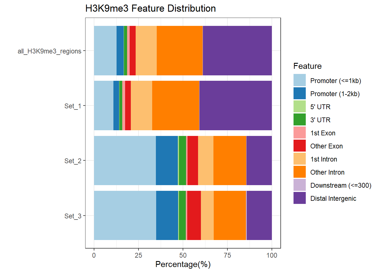
| Version | Author | Date |
|---|---|---|
| 1a7940a | reneeisnowhere | 2025-09-03 |
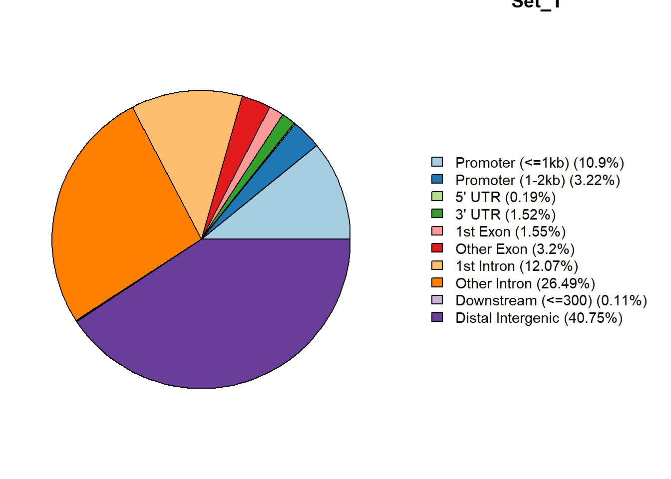
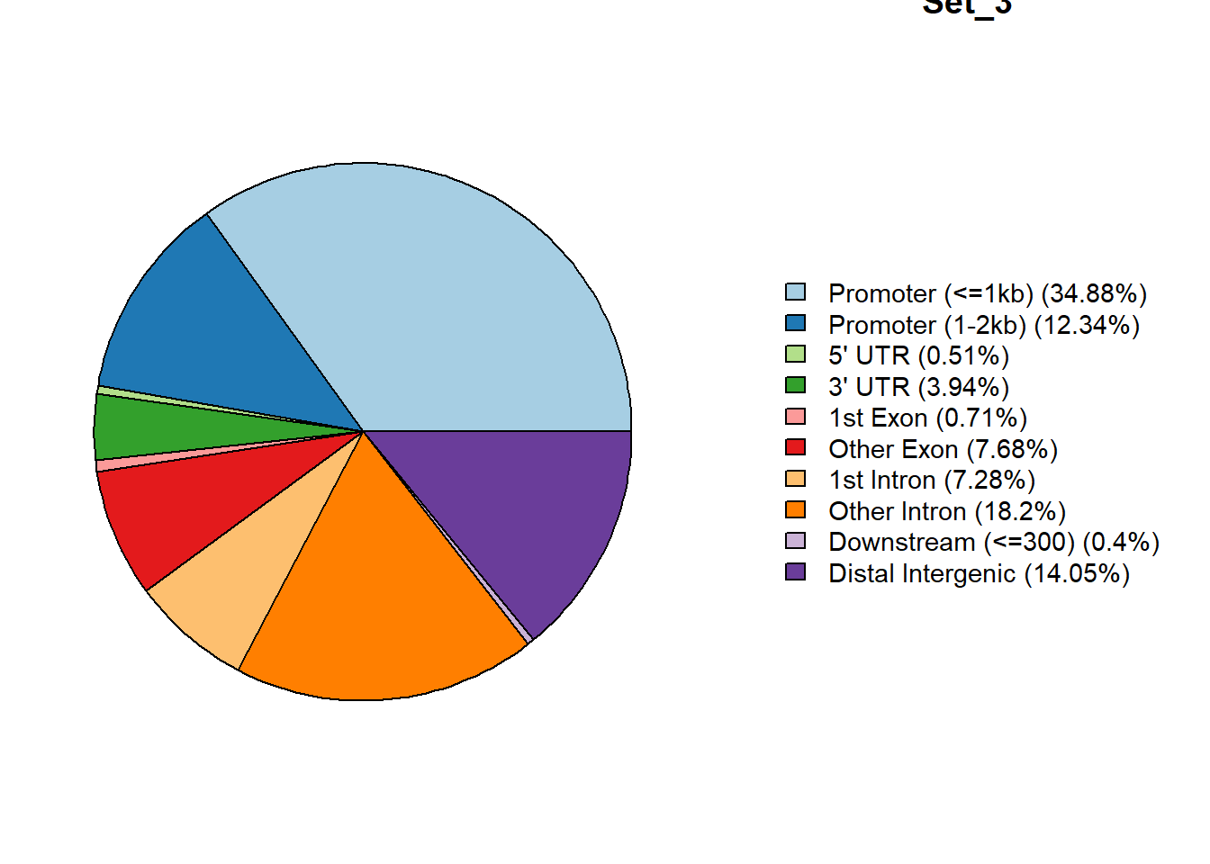
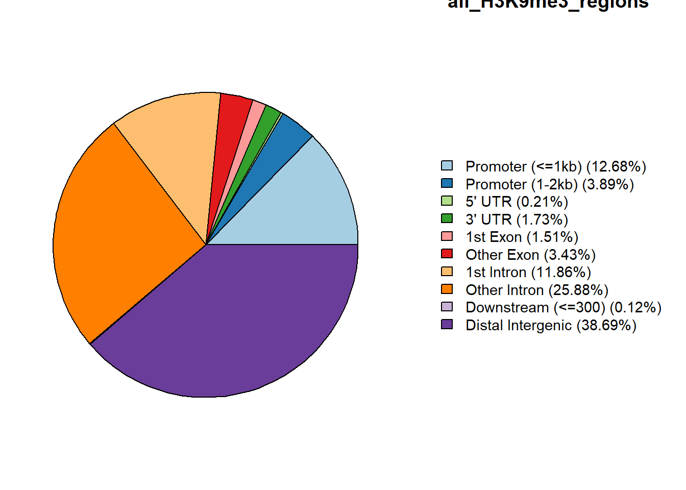
# pie_plots_H3K9me3 <-   map(peakAnnoList_H3K9me3, ~ plotAnnoPie(.x))
for(nm in names(peakAnnoList_H3K9me3)) {
  plotAnnoPie(peakAnnoList_H3K9me3[[nm]])
  title(main = nm)  # base R title
}
| Version | Author | Date |
|---|---|---|
| 1a7940a | reneeisnowhere | 2025-09-03 |

| Version | Author | Date |
|---|---|---|
| 1a7940a | reneeisnowhere | 2025-09-03 |
| Version | Author | Date |
|---|---|---|
| 1a7940a | reneeisnowhere | 2025-09-03 |
| Version | Author | Date |
|---|---|---|
| 1a7940a | reneeisnowhere | 2025-09-03 |
Histone proportions
H3K9me3_lookup <- imap_dfr(peakAnnoList_H3K9me3[1:3], ~
  tibble(Peakid = .x@anno$Peakid, cluster = .y))
all_H3K9me3_regions %>%
  mutate(group="H3K9me3") %>%
  left_join(., H3K9me3_lookup) %>%
   tidyr::replace_na(list(cluster = "NA")) %>%
  ggplot(., aes(y=group,fill=cluster))+
  geom_bar()+
  geom_text(aes( label = scales::percent(..prop..),
                   x= ..prop.. ), stat= "count", vjust = -.5)+
  ggtitle("H3K9me3 proportions of ROIs")+
  theme_classic()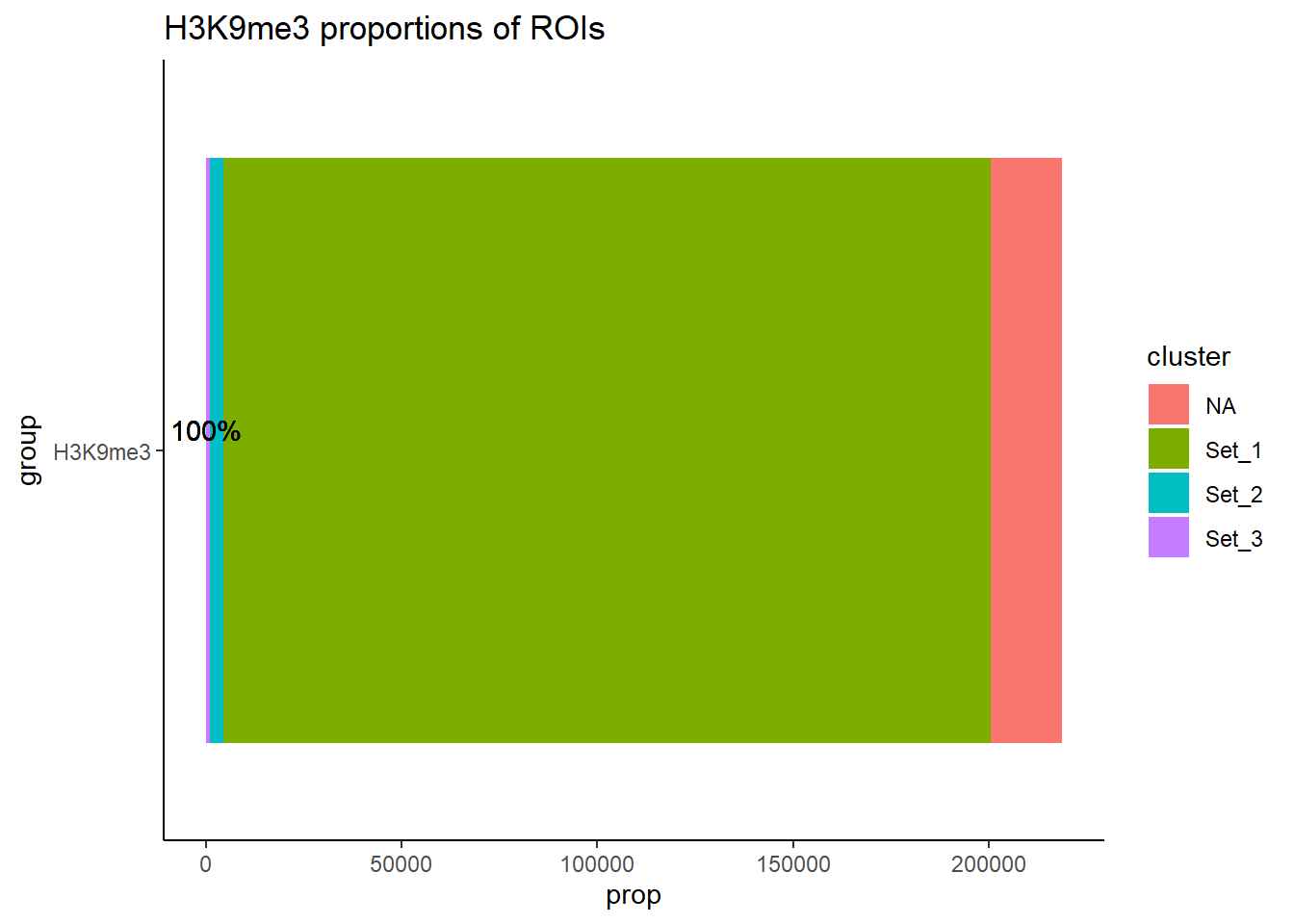
all_H3K9me3_regions %>%
  mutate(group="H3K9me3") %>%
  left_join(., H3K9me3_lookup) %>%
   tidyr::replace_na(list(cluster = "NA")) %>%
  mutate(cluster=factor(cluster, levels = c("Set_1","Set_2","Set_3","NA"))) %>%
  ggplot(., aes(x=cluster,y = after_stat(prop), group=1))+
  geom_bar(aes(stat="count"))+
  geom_text(aes( label = scales::percent(after_stat(prop))),
            stat= "count", vjust = -.5)+
  scale_y_continuous(
    labels = scales::percent,
    expand = expansion(mult = c(0, 0.1))
  ) +
  ggtitle("H3K9me3 proportions of ROIs")+
  theme_classic()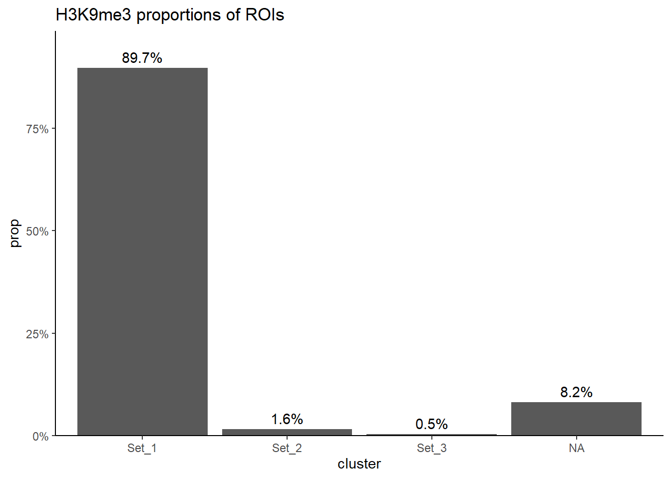
all_H3K9me3_regions %>%
  mutate(group="H3K9me3") %>%
  left_join(., H3K9me3_lookup) %>%
   tidyr::replace_na(list(cluster = "NA")) %>%
  group_by(cluster) %>%
  tally(name = "n_ROIs") %>%
  ungroup() %>%
  DT::datatable(
    rownames = FALSE,
    caption = htmltools::tags$caption(
      style = "caption-side: top; text-align: left;",
      "H3K9me3 ROI counts per cluster"
    ),
    options = list(
      pageLength = 10,
      autoWidth = TRUE,
      dom = "tip"
    )
  )
LFC H3K9me3
Set1
# H3K9me3_toptable_list %>%
#   dplyr::filter(genes %in% H3K9me3_set1$.) %>%
#   dplyr::select(group,genes,logFC) %>%
#   mutate(group=factor(group, levels = c("H3K9me3_24T","H3K9me3_24R","H3K9me3_144R"))) %>%
#   ggplot(., aes(x=group, y=logFC))+
#   geom_boxplot(aes(fill=group))+
#   geom_signif(comparisons = list(c("H3K9me3_24T", "H3K9me3_144R"),
#                                  c("H3K9me3_24T","H3K9me3_24R"),
#                                  c("H3K9me3_24R", "H3K9me3_144R")),
#                               step_increase = 0.1,
#               map_signif_level = FALSE,
#               test = "wilcox.test")+
#   theme_bw()+
#   ggtitle("LFC across time for H3K9me3 set1")


H3K9me3_toptable_list %>%
  dplyr::filter(genes %in% H3K9me3_set1$.) %>%
  dplyr::select(group,genes,logFC) %>%
  mutate(group=factor(group, levels = c("H3K9me3_24T","H3K9me3_24R","H3K9me3_144R")),
         logFC=abs(logFC)) %>%
  ggplot(., aes(x=group, y=logFC))+
  geom_boxplot(aes(fill=group))+
  geom_signif(comparisons = list(c("H3K9me3_24T", "H3K9me3_144R"),
                                 c("H3K9me3_24T","H3K9me3_24R"),
                                 c("H3K9me3_24R", "H3K9me3_144R")),
                              step_increase = 0.1,
              map_signif_level = FALSE,
              test = "wilcox.test")+
  theme_bw()+
  ggtitle("Absolute LFC across time for H3K9me3 set1")
| Version | Author | Date |
|---|---|---|
| 1a7940a | reneeisnowhere | 2025-09-03 |
  set1_9me3 <- H3K9me3_toptable_list %>%
  dplyr::filter(genes %in% H3K9me3_set1$.) %>%
  dplyr::select(group,genes,logFC) %>%
   mutate(group=factor(group, levels = c("H3K9me3_24T","H3K9me3_24R","H3K9me3_144R")),
         logFC=abs(logFC)) %>%
  group_by(group) %>%
  summarize(med_Set1=median(logFC),.groups="drop")
set2
# H3K9me3_toptable_list %>%
#   dplyr::filter(genes %in% H3K9me3_set2$.) %>%
#   dplyr::select(group,genes,logFC) %>%
#   mutate(group=factor(group, levels = c("H3K9me3_24T","H3K9me3_24R","H3K9me3_144R"))) %>%
#   ggplot(., aes(x=group, y=logFC))+
#   geom_boxplot(aes(fill=group))+
#   geom_signif(comparisons = list(c("H3K9me3_24T", "H3K9me3_144R"),
#                                  c("H3K9me3_24T","H3K9me3_24R"),
#                                  c("H3K9me3_24R", "H3K9me3_144R")),
#                               step_increase = 0.1,
#               map_signif_level = FALSE,
#               test = "wilcox.test")+
#   theme_bw()+
#   ggtitle("LFC across time for H3K9me3 set2")


H3K9me3_toptable_list %>%
  dplyr::filter(genes %in% H3K9me3_set2$.) %>%
  dplyr::select(group,genes,logFC) %>%
  mutate(group=factor(group, levels = c("H3K9me3_24T","H3K9me3_24R","H3K9me3_144R")),
         logFC=abs(logFC)) %>%
  ggplot(., aes(x=group, y=logFC))+
  geom_boxplot(aes(fill=group))+
  geom_signif(comparisons = list(c("H3K9me3_24T", "H3K9me3_144R"),
                                 c("H3K9me3_24T","H3K9me3_24R"),
                                 c("H3K9me3_24R", "H3K9me3_144R")),
                              step_increase = 0.1,
              map_signif_level = FALSE,
              test = "wilcox.test")+
  theme_bw()+
  ggtitle("Absolute LFC across time for H3K9me3 set2")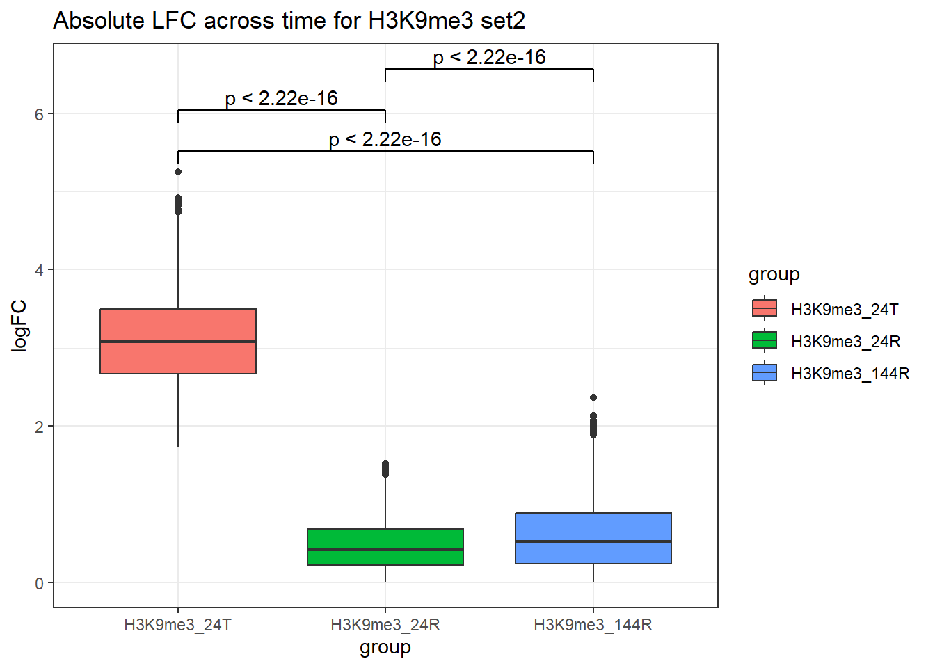
| Version | Author | Date |
|---|---|---|
| 1a7940a | reneeisnowhere | 2025-09-03 |
  set2_9me3 <- H3K9me3_toptable_list %>%
  dplyr::filter(genes %in% H3K9me3_set2$.) %>%
  dplyr::select(group,genes,logFC) %>%
   mutate(group=factor(group, levels = c("H3K9me3_24T","H3K9me3_24R","H3K9me3_144R")),
         logFC=abs(logFC)) %>%
  group_by(group) %>%
  summarize(med_Set2=median(logFC),.groups="drop")
set3
# H3K9me3_toptable_list %>%
#   dplyr::filter(genes %in% H3K9me3_set3$.) %>%
#   dplyr::select(group,genes,logFC) %>%
#   mutate(group=factor(group, levels = c("H3K9me3_24T","H3K9me3_24R","H3K9me3_144R"))) %>%
#   ggplot(., aes(x=group, y=logFC))+
#   geom_boxplot(aes(fill=group))+
#   geom_signif(comparisons = list(c("H3K9me3_24T", "H3K9me3_144R"),
#                                  c("H3K9me3_24T","H3K9me3_24R"),
#                                  c("H3K9me3_24R", "H3K9me3_144R")),
#                               step_increase = 0.1,
#               map_signif_level = FALSE,
#               test = "wilcox.test")+
#   theme_bw()+
#   ggtitle("LFC across time for H3K9me3 set3")


H3K9me3_toptable_list %>%
  dplyr::filter(genes %in% H3K9me3_set3$.) %>%
  dplyr::select(group,genes,logFC) %>%
  mutate(group=factor(group, levels = c("H3K9me3_24T","H3K9me3_24R","H3K9me3_144R")),
         logFC=abs(logFC)) %>%
  ggplot(., aes(x=group, y=logFC))+
  geom_boxplot(aes(fill=group))+
  geom_signif(comparisons = list(c("H3K9me3_24T", "H3K9me3_144R"),
                                 c("H3K9me3_24T","H3K9me3_24R"),
                                 c("H3K9me3_24R", "H3K9me3_144R")),
                              step_increase = 0.1,
              map_signif_level = FALSE,
              test = "wilcox.test")+
  theme_bw()+
  ggtitle("Absolute LFC across time for H3K9me3 set3")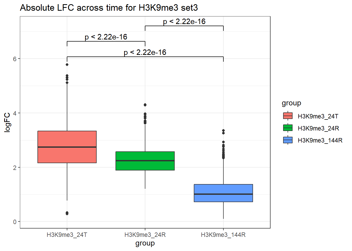
| Version | Author | Date |
|---|---|---|
| 1a7940a | reneeisnowhere | 2025-09-03 |
  H3K9me3_toptable_list %>%
  dplyr::filter(genes %in% H3K9me3_set3$.) %>%
  dplyr::select(group,genes,logFC) %>%
  mutate(group=factor(group, levels = c("H3K9me3_24T","H3K9me3_24R","H3K9me3_144R")),
         logFC=abs(logFC)) %>%
  group_by(group) %>%
  summarize(med_Set3=median(logFC),.groups="drop") %>%
  left_join(set1_9me3, by="group") %>%
  left_join(set2_9me3, by="group") %>%
  pivot_longer(cols=!group, values_to = "median_LFC", names_to = "set") %>%
  ggplot(., aes(x=group, y=median_LFC, group=set, color=set))+
  geom_point(size=4)+
  geom_line(aes(alpha = 0.8, linewidth=3))+
  theme_bw()+
  ggtitle("LFC across time for H3K9me3 sets")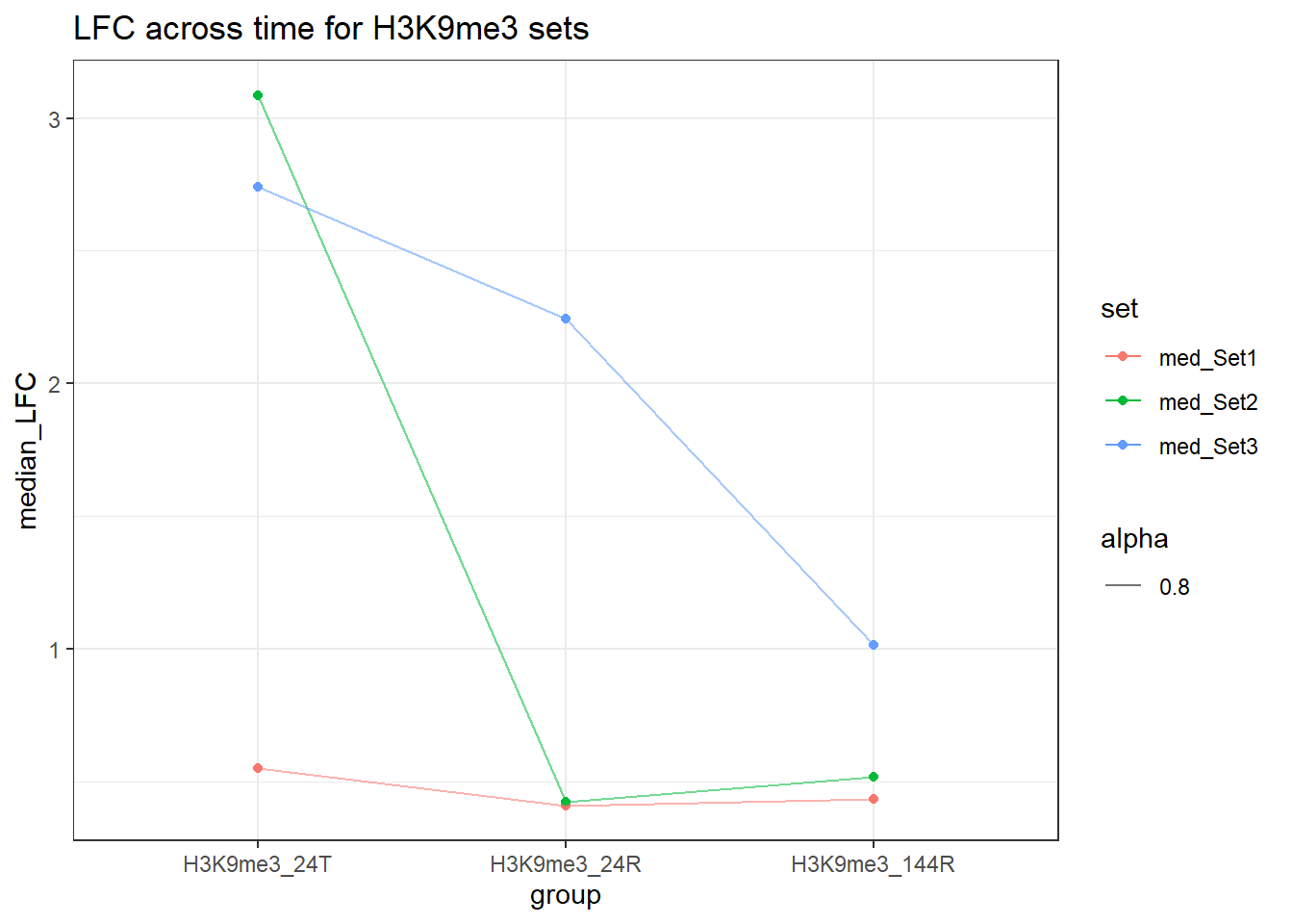
Top 100
This is the calculation of Top 100 in each category, then united
cormotif_initial_H3K9me3 <- readRDS("data/Cormotif_data/Cormotif_initial_H3K9me3.RDS")
row.names(cormotif_initial_H3K9me3$bestmotif$clustlike) <- row.names(H3K9me3_filt_lcpm)
H3K9me3_clustlike <- cormotif_initial_H3K9me3$bestmotif$clustlike %>%
  as.data.frame() %>%
  rownames_to_column("Peakid")

H3K9me3_clusters <- list(
  Set1="V1",
  Set2="V2",
  Set3="V3")


Sets_H3K9me3 <- H3K9me3_toptable_list %>%
  mutate(cluster=case_when(genes %in% H3K9me3_set1$. ~ "Set1",
                           genes %in% H3K9me3_set2$. ~ "Set2",
                           genes %in% H3K9me3_set3$. ~ "Set3",
                           TRUE ~ "not_assigned")) %>%
  left_join(., H3K9me3_clustlike,by=c("genes"="Peakid")) %>%
  dplyr::filter(cluster!="not_assigned")

###This code uses the H3K9me3_clusters list and filters through Sets_H3K9me3 data frame by selecting
Sets_H3K9me3_top <- map_dfr(names(H3K9me3_clusters), function(cl) {
  col <- H3K9me3_clusters[[cl]]
  Sets_H3K9me3 %>%
    filter(cluster == cl) %>%
    # group_by(group) %>%
    slice_max(order_by = .data[[col]], n = 100)
}) %>%
  ungroup()

## now plot

Sets_H3K9me3_top %>%
  mutate(group=factor(group, levels = c("H3K9me3_24T","H3K9me3_24R","H3K9me3_144R")),
         cluster=factor(cluster, levels=c("Set1","Set2","Set3"))) %>%
  ggplot(., aes(x= group,y = logFC, group = interaction(cluster, genes), color=cluster))+
  geom_point()+
  geom_line(aes(alpha = 0.8))+
  theme_bw()+
  facet_wrap(~cluster)+
  ggtitle("LFC across time for H3K9me3 top 100 by Set")+
  theme(axis.text.x = element_text(angle=90) )
| Version | Author | Date |
|---|---|---|
| 1ce5e71 | reneeisnowhere | 2025-09-16 |
# saveRDS(Sets_H3K9me3_top,"data/motif_lists/H3K9me3_toplistbymotif.RDS")peakAnnoList_H3K36me3 <- readRDS("data/motif_lists/H3K36me3_annotated_peaks.RDS")
out_dir <- "data/Bed_exports/H3K36me3_sets"
set_list <- names(peakAnnoList_H3K36me3)
for (group_name in set_list) {
cs <- peakAnnoList_H3K36me3[[group_name]]
gr <- cs@anno
# Set BED name column
mcols(gr)$name <- mcols(gr)$Peakid
# Optional: if you want a score column
if(!"score" %in% colnames(mcols(gr))) {
mcols(gr)$score <- 0
}
# Export to BED
bed_file <- file.path(out_dir, paste0(group_name, "_H3K36me3_ROI.bed"))
# Export
export(gr, bed_file, format = "BED")
cat("Exported:", bed_file, "\n")
}
sessionInfo()R version 4.4.2 (2024-10-31 ucrt)
Platform: x86_64-w64-mingw32/x64
Running under: Windows 11 x64 (build 26200)
Matrix products: default
locale:
[1] LC_COLLATE=English_United States.utf8
[2] LC_CTYPE=English_United States.utf8
[3] LC_MONETARY=English_United States.utf8
[4] LC_NUMERIC=C
[5] LC_TIME=English_United States.utf8
time zone: America/Chicago
tzcode source: internal
attached base packages:
[1] stats4 grid stats graphics grDevices utils datasets
[8] methods base
other attached packages:
[1] ChIPseeker_1.42.1
[2] TxDb.Hsapiens.UCSC.hg38.knownGene_3.20.0
[3] GenomicFeatures_1.58.0
[4] AnnotationDbi_1.68.0
[5] Biobase_2.66.0
[6] BiocParallel_1.40.2
[7] ggsignif_0.6.4
[8] ggVennDiagram_1.5.4
[9] smplot2_0.2.5
[10] cowplot_1.2.0
[11] ggrastr_1.0.2
[12] Rsubread_2.20.0
[13] gcplyr_1.12.0
[14] ggpmisc_0.6.2
[15] ggpp_0.5.9
[16] corrplot_0.95
[17] ggpubr_0.6.1
[18] GenomicRanges_1.58.0
[19] GenomeInfoDb_1.42.3
[20] IRanges_2.40.1
[21] S4Vectors_0.44.0
[22] BiocGenerics_0.52.0
[23] genomation_1.38.0
[24] kableExtra_1.4.0
[25] DT_0.33
[26] viridis_0.6.5
[27] viridisLite_0.4.2
[28] data.table_1.17.8
[29] ComplexHeatmap_2.22.0
[30] edgeR_4.4.2
[31] limma_3.62.2
[32] lubridate_1.9.4
[33] forcats_1.0.0
[34] stringr_1.5.1
[35] dplyr_1.1.4
[36] purrr_1.1.0
[37] readr_2.1.5
[38] tidyr_1.3.1
[39] tibble_3.3.0
[40] ggplot2_3.5.2
[41] tidyverse_2.0.0
[42] workflowr_1.7.1
loaded via a namespace (and not attached):
[1] fs_1.6.6
[2] matrixStats_1.5.0
[3] bitops_1.0-9
[4] enrichplot_1.26.6
[5] httr_1.4.7
[6] RColorBrewer_1.1-3
[7] doParallel_1.0.17
[8] tools_4.4.2
[9] backports_1.5.0
[10] R6_2.6.1
[11] lazyeval_0.2.2
[12] GetoptLong_1.0.5
[13] withr_3.0.2
[14] gridExtra_2.3
[15] quantreg_6.1
[16] cli_3.6.5
[17] textshaping_1.0.1
[18] labeling_0.4.3
[19] sass_0.4.10
[20] Rsamtools_2.22.0
[21] systemfonts_1.2.3
[22] yulab.utils_0.2.1
[23] foreign_0.8-90
[24] DOSE_4.0.1
[25] svglite_2.2.1
[26] R.utils_2.13.0
[27] dichromat_2.0-0.1
[28] plotrix_3.8-4
[29] BSgenome_1.74.0
[30] pwr_1.3-0
[31] rstudioapi_0.17.1
[32] impute_1.80.0
[33] RSQLite_2.4.3
[34] generics_0.1.4
[35] gridGraphics_0.5-1
[36] TxDb.Hsapiens.UCSC.hg19.knownGene_3.2.2
[37] shape_1.4.6.1
[38] BiocIO_1.16.0
[39] crosstalk_1.2.2
[40] vroom_1.6.5
[41] gtools_3.9.5
[42] car_3.1-3
[43] GO.db_3.20.0
[44] Matrix_1.7-3
[45] ggbeeswarm_0.7.2
[46] abind_1.4-8
[47] R.methodsS3_1.8.2
[48] lifecycle_1.0.4
[49] whisker_0.4.1
[50] yaml_2.3.10
[51] carData_3.0-5
[52] SummarizedExperiment_1.36.0
[53] gplots_3.2.0
[54] qvalue_2.38.0
[55] SparseArray_1.6.2
[56] blob_1.2.4
[57] promises_1.3.3
[58] crayon_1.5.3
[59] ggtangle_0.0.7
[60] lattice_0.22-7
[61] KEGGREST_1.46.0
[62] pillar_1.11.0
[63] knitr_1.50
[64] fgsea_1.32.4
[65] rjson_0.2.23
[66] boot_1.3-32
[67] codetools_0.2-20
[68] fastmatch_1.1-6
[69] glue_1.8.0
[70] getPass_0.2-4
[71] ggfun_0.2.0
[72] treeio_1.30.0
[73] vctrs_0.6.5
[74] png_0.1-8
[75] gtable_0.3.6
[76] cachem_1.1.0
[77] xfun_0.52
[78] S4Arrays_1.6.0
[79] survival_3.8-3
[80] iterators_1.0.14
[81] statmod_1.5.0
[82] nlme_3.1-168
[83] ggtree_3.14.0
[84] bit64_4.6.0-1
[85] rprojroot_2.1.1
[86] bslib_0.9.0
[87] vipor_0.4.7
[88] KernSmooth_2.23-26
[89] rpart_4.1.24
[90] colorspace_2.1-1
[91] DBI_1.2.3
[92] Hmisc_5.2-3
[93] seqPattern_1.38.0
[94] nnet_7.3-20
[95] tidyselect_1.2.1
[96] processx_3.8.6
[97] bit_4.6.0
[98] compiler_4.4.2
[99] curl_7.0.0
[100] git2r_0.36.2
[101] htmlTable_2.4.3
[102] SparseM_1.84-2
[103] xml2_1.4.0
[104] DelayedArray_0.32.0
[105] rtracklayer_1.66.0
[106] caTools_1.18.3
[107] checkmate_2.3.3
[108] scales_1.4.0
[109] callr_3.7.6
[110] rappdirs_0.3.3
[111] digest_0.6.37
[112] rmarkdown_2.29
[113] XVector_0.46.0
[114] htmltools_0.5.8.1
[115] pkgconfig_2.0.3
[116] base64enc_0.1-3
[117] MatrixGenerics_1.18.1
[118] fastmap_1.2.0
[119] rlang_1.1.6
[120] GlobalOptions_0.1.2
[121] htmlwidgets_1.6.4
[122] UCSC.utils_1.2.0
[123] farver_2.1.2
[124] jquerylib_0.1.4
[125] zoo_1.8-14
[126] jsonlite_2.0.0
[127] GOSemSim_2.32.0
[128] R.oo_1.27.1
[129] RCurl_1.98-1.17
[130] magrittr_2.0.3
[131] polynom_1.4-1
[132] Formula_1.2-5
[133] GenomeInfoDbData_1.2.13
[134] ggplotify_0.1.2
[135] patchwork_1.3.2
[136] Rcpp_1.1.0
[137] ape_5.8-1
[138] stringi_1.8.7
[139] zlibbioc_1.52.0
[140] MASS_7.3-65
[141] plyr_1.8.9
[142] ggrepel_0.9.6
[143] parallel_4.4.2
[144] Biostrings_2.74.1
[145] splines_4.4.2
[146] hms_1.1.3
[147] circlize_0.4.16
[148] locfit_1.5-9.12
[149] ps_1.9.1
[150] igraph_2.1.4
[151] reshape2_1.4.4
[152] XML_3.99-0.18
[153] evaluate_1.0.5
[154] tzdb_0.5.0
[155] foreach_1.5.2
[156] httpuv_1.6.16
[157] MatrixModels_0.5-4
[158] clue_0.3-66
[159] gridBase_0.4-7
[160] broom_1.0.9
[161] restfulr_0.0.16
[162] tidytree_0.4.6
[163] rstatix_0.7.2
[164] later_1.4.2
[165] aplot_0.2.8
[166] memoise_2.0.1
[167] beeswarm_0.4.0
[168] GenomicAlignments_1.42.0
[169] cluster_2.1.8.1
[170] timechange_0.3.0