H3K27me3 and TE overlap
Renee Matthews
2026-03-17
Last updated: 2026-03-17
Checks: 7 0
Knit directory: DXR_continue/
This reproducible R Markdown analysis was created with workflowr (version 1.7.1). The Checks tab describes the reproducibility checks that were applied when the results were created. The Past versions tab lists the development history.
Great! Since the R Markdown file has been committed to the Git repository, you know the exact version of the code that produced these results.
Great job! The global environment was empty. Objects defined in the global environment can affect the analysis in your R Markdown file in unknown ways. For reproduciblity it’s best to always run the code in an empty environment.
The command set.seed(20250701) was run prior to running
the code in the R Markdown file. Setting a seed ensures that any results
that rely on randomness, e.g. subsampling or permutations, are
reproducible.
Great job! Recording the operating system, R version, and package versions is critical for reproducibility.
Nice! There were no cached chunks for this analysis, so you can be confident that you successfully produced the results during this run.
Great job! Using relative paths to the files within your workflowr project makes it easier to run your code on other machines.
Great! You are using Git for version control. Tracking code development and connecting the code version to the results is critical for reproducibility.
The results in this page were generated with repository version d22c09b. See the Past versions tab to see a history of the changes made to the R Markdown and HTML files.
Note that you need to be careful to ensure that all relevant files for
the analysis have been committed to Git prior to generating the results
(you can use wflow_publish or
wflow_git_commit). workflowr only checks the R Markdown
file, but you know if there are other scripts or data files that it
depends on. Below is the status of the Git repository when the results
were generated:
Ignored files:
    Ignored:    .Rhistory
    Ignored:    .Rproj.user/
    Ignored:    data/Bed_exports/
    Ignored:    data/Cormotif_data/
    Ignored:    data/DER_data/
    Ignored:    data/Other_paper_data/
    Ignored:    data/RDS_files/
    Ignored:    data/TE_annotation/
    Ignored:    data/alignment_summary.txt
    Ignored:    data/all_peak_final_dataframe.txt
    Ignored:    data/cell_line_info_.tsv
    Ignored:    data/full_summary_QC_metrics.txt
    Ignored:    data/motif_lists/
    Ignored:    data/number_frag_peaks_summary.txt

Untracked files:
    Untracked:  H3K27ac_all_regions_test.bed
    Untracked:  H3K27ac_consensus_clusters_test.bed
    Untracked:  analysis/GREAT_H3K27ac.Rmd
    Untracked:  analysis/H3K27ac_ChromHMM_FC.Rmd
    Untracked:  analysis/H3K27me3_TE_investigation.Rmd
    Untracked:  analysis/H3K36me3_TE_investigation.Rmd
    Untracked:  analysis/Top2a_Top2b_expression.Rmd
    Untracked:  analysis/computeMatrixplots.Rmd
    Untracked:  analysis/maps_and_plots.Rmd
    Untracked:  analysis/proteomics.Rmd
    Untracked:  code/For_john.R
    Untracked:  other_analysis/

Unstaged changes:
    Modified:   analysis/H3K27_TE_overlap.Rmd
    Modified:   analysis/H3K27ac_cisRE.Rmd
    Modified:   analysis/H3K27ac_summit_processing.Rmd
    Modified:   analysis/H3K27me3_summit_processing.Rmd
    Modified:   analysis/H3K36me3_summit_processing.Rmd
    Modified:   analysis/H3K9me3_TE_investigation.Rmd
    Modified:   analysis/chromHMM.Rmd
    Modified:   analysis/dual_histone_TE_investigation.Rmd
    Modified:   analysis/summit_files_processing.Rmd
Note that any generated files, e.g. HTML, png, CSS, etc., are not included in this status report because it is ok for generated content to have uncommitted changes.
These are the previous versions of the repository in which changes were
made to the R Markdown (analysis/H3K27me3_TE_overlap.Rmd)
and HTML (docs/H3K27me3_TE_overlap.html) files. If you’ve
configured a remote Git repository (see ?wflow_git_remote),
click on the hyperlinks in the table below to view the files as they
were in that past version.
| File | Version | Author | Date | Message |
|---|---|---|---|---|
| Rmd | d22c09b | reneeisnowhere | 2026-03-17 | adding in LTR examination |
| html | ba7cf29 | reneeisnowhere | 2026-01-27 | Build site. |
| Rmd | fbfe34d | reneeisnowhere | 2026-01-27 | adding full ROI to summit page for enrichment checks |
| html | 8f7ef07 | reneeisnowhere | 2026-01-26 | Build site. |
| Rmd | a44db38 | reneeisnowhere | 2026-01-26 | new overlaps autosomal only |
| html | 177cb71 | reneeisnowhere | 2026-01-23 | Build site. |
| Rmd | e8e2585 | reneeisnowhere | 2026-01-23 | image update |
library(tidyverse)
library(GenomicRanges)
library(plyranges)
library(genomation)
library(readr)
library(rtracklayer)
library(stringr)
library(ggrepel)
library(DT)
First steps: breakdown repeatmasker into groups and pull out the ones by each class I am interested in.
autosomes <- paste0("chr", 1:22)
repeatmasker <- read_delim("data/Other_paper_data/repeatmasker_20250911.txt",
    delim = "\t", escape_double = FALSE,
    trim_ws = TRUE)
colnames(repeatmasker)
[1] "#bin" "swScore" "milliDiv" "milliDel" "milliIns" "genoName"
[7] "genoStart" "genoEnd" "genoLeft" "strand" "repName" "repClass"
[13] "repFamily" "repStart" "repEnd" "repLeft" "id" repeatmasker_clean <- repeatmasker %>% mutate(
strand = ifelse(strand == "C", "-", "+")
) %>%
mutate(
start = genoStart + 1,
end = genoEnd)%>%
mutate(repFamily= str_remove(repFamily, "\\?$")) %>%
dplyr::filter(genoName %in% autosomes) %>%
mutate(RM_id=paste0(genoName,":",start,"-",end,":",id))
rpt_split <- split(repeatmasker_clean, repeatmasker_clean$repClass)
rpt_split_gr_list <- lapply(rpt_split, function(df) {
GRanges(
seqnames = df$genoName,
ranges = IRanges(start = df$start, end = df$end),
strand = df$strand,
repName = df$repName,
repClass = df$repClass,
repFamily = df$repFamily,
swScore = df$swScore,
milliDiv = df$milliDiv,
milliDel = df$milliDel,
milliIns = df$milliIns,
RM_id = df$RM_id
)
})
rmskr_std_gr <- GRanges(
seqnames = repeatmasker_clean$genoName,
ranges = IRanges(
start = repeatmasker_clean$start,
end = repeatmasker_clean$end
),
strand = repeatmasker_clean$strand,
repName = repeatmasker_clean$repName,
repClass = repeatmasker_clean$repClass,
repFamily = repeatmasker_clean$repFamily,
swScore = repeatmasker_clean$swScore,
milliDiv = repeatmasker_clean$milliDiv,
milliDel = repeatmasker_clean$milliDel,
milliIns = repeatmasker_clean$milliIns,
id = repeatmasker_clean$RM_id
)SINE_gr <- rpt_split_gr_list$SINE
SINE_df <- SINE_gr %>%
as.data.frame()
SINE_split_df <- split(SINE_df, SINE_df$repFamily)
LINE_gr <- rpt_split_gr_list$LINE
LINE_df <- LINE_gr %>%
as.data.frame()
LINE_split_df <- split(LINE_df, LINE_df$repFamily)
LTR_gr <- rpt_split_gr_list$LTR
LTR_df <- LTR_gr %>%
as.data.frame()
LTR_split_df <- split(LTR_df, LTR_df$repFamily)
SVA_gr <- rpt_split_gr_list$Retroposon
SVA_df <- SVA_gr %>%
as.data.frame()
SVA_split_df <- split(SVA_df, SVA_df$repFamily)
DNA_gr <- rpt_split_gr_list$DNA
DNA_df <- DNA_gr %>%
as.data.frame()
DNA_split_df <- split(DNA_df, DNA_df$repFamily)H3K27me3_summit_gr <- readRDS("data/RDS_files/H3K27me3_complete_summit_gr.RDS")
peakAnnoList_H3K27me3 <- readRDS("data/motif_lists/H3K27me3_annotated_peaks.RDS")
H3K27me3_lookup <- imap_dfr(peakAnnoList_H3K27me3[1:3], ~
tibble(Peakid = .x@anno$Peakid, cluster = .y)
)
H3K27me3_sets_gr <- lapply(peakAnnoList_H3K27me3, function(df) {
as_granges(df)
})
##assigning Peakid as name of summit region
mcols(H3K27me3_summit_gr)$name <- mcols(H3K27me3_summit_gr)$Peakid
comparisons <- tibble(
cluster2 = c("Set_2"),
cluster1 = c("Set_1")
)# Generic pairwise Fisher test
test_pair_TE_generic <- function(df_long, te_name, cluster1, cluster2) {
sub_df <- df_long %>%
filter(TE_type == te_name) %>%
complete(
cluster = c(cluster1, cluster2),
status = c("TE", "not_TE"),
fill = list(count = 0))
# enforce fixed order
status_levels <- c("TE", "not_TE")
# assume "status" column has TE vs wnot_TE automatically
statuses <- unique(sub_df$status)
if(length(statuses) != 2) {
# ensure we have exactly two categories, fill missing with 0
sub_df <- sub_df %>%
complete(cluster, status, fill = list(count = 0))
statuses <- unique(sub_df$status)
}
# extract counts for cluster1
c1_counts <- sub_df %>%
filter(cluster == cluster1) %>%
arrange(factor(status, levels = status_levels)) %>% # ensure same order
pull(count)
# extract counts for cluster2
c2_counts <- sub_df %>%
filter(cluster == cluster2) %>%
arrange(factor(status, levels = status_levels)) %>%
pull(count)
# build 2x2 matrix
mat <- matrix(
c(c2_counts, c1_counts),
nrow = 2,
byrow = TRUE,
dimnames = list(
cluster = c(cluster2, cluster1),
category = status_levels
)
)
ft <- tryCatch(
fisher.test(mat, workspace = 2e8),
error = function(e) fisher.test(mat, simulate.p.value = TRUE, B = 1e5)
)
tibble(
TE_type = te_name,
comparison = paste(cluster2, "vs", cluster1),
odds_ratio = ft$estimate,
lower_CI = ft$conf.int[1],
upper_CI = ft$conf.int[2],
p_value = ft$p.value
)
}test_pair_TE_repName <- function(df_long, rep_name, cluster1, cluster2) {
# Subset for the specific repName
sub_df <- df_long %>%
filter(repName == rep_name) %>%
complete(
cluster = c(cluster1, cluster2),
status = c("TE", "not_TE"),
fill = list(count = 0)
)
# fixed order of statuses
status_levels <- c("TE", "not_TE")
# make sure both statuses exist
statuses <- unique(sub_df$status)
if(length(statuses) != 2) {
sub_df <- sub_df %>%
complete(cluster, status, fill = list(count = 0))
statuses <- unique(sub_df$status)
}
# counts for cluster1
c1_counts <- sub_df %>%
filter(cluster == cluster1) %>%
arrange(factor(status, levels = status_levels)) %>%
pull(count)
# counts for cluster2
c2_counts <- sub_df %>%
filter(cluster == cluster2) %>%
arrange(factor(status, levels = status_levels)) %>%
pull(count)
# 2x2 matrix for Fisher test
mat <- matrix(
c(c2_counts, c1_counts),
nrow = 2,
byrow = TRUE,
dimnames = list(
cluster = c(cluster2, cluster1),
category = status_levels
)
)
ft <- tryCatch(
fisher.test(mat, workspace = 2e8),
error = function(e) fisher.test(mat, simulate.p.value = TRUE, B = 1e5)
)
tibble(
repName = rep_name,
comparison = paste(cluster2, "vs", cluster1),
odds_ratio = ft$estimate,
lower_CI = ft$conf.int[1],
upper_CI = ft$conf.int[2],
p_value = ft$p.value
)
}All H3K27me3 ROIs overlapping a TE at summits
overlapping summits and all TEs dataframe making:
dataf <- H3K27me3_summit_gr
# H3K27me3_summit_ols <-

   # 1️⃣ find overlaps
  hits <- findOverlaps(dataf, rmskr_std_gr)

  if (length(hits) == 0) {
  H3K27me3_summit_ols <- tibble()
} else {

  H3K27me3_summit_ols <- tibble(
    Peakid     = dataf$Peakid[queryHits(hits)],
    cluster    = dataf$cluster[queryHits(hits)],
    seqnames   = as.character(seqnames(dataf))[queryHits(hits)],
    summit_pos = start(dataf)[queryHits(hits)],

    repName   = rmskr_std_gr$repName[subjectHits(hits)],
    repFamily = rmskr_std_gr$repFamily[subjectHits(hits)],
    repClass  = rmskr_std_gr$repClass[subjectHits(hits)],
    milliDiv  = rmskr_std_gr$milliDiv[subjectHits(hits)],
    milliDel  = rmskr_std_gr$milliDel[subjectHits(hits)],
    milliIns  = rmskr_std_gr$milliIns[subjectHits(hits)],
    ID  = rmskr_std_gr$id[subjectHits(hits)]
  )
}
# rmskr_nonoverlapping_H3K27me3_gr <- rmskr_std_gr[countOverlaps(rmskr_std_gr, H3K27me3_sets_gr[[4]]) == 0]

H3K27me3_summit_Peakids <- H3K27me3_summit_ols %>%
    distinct(Peakid)
  # saveRDS(H3K27me3_summit_ols,"data/RDS_files/H3K27me3_summit_ROI_TE_overlaps.RDS")

H3K27me3_summit_df <- readRDS("data/RDS_files/H3K27me3_complete_summit_df.RDS")
making summit TE overlap annotation dataframe
all_summits_df <-
H3K27me3_summit_df %>%
  mutate(summit_id=paste0(roi_seqname,":",summit_pos)) %>%
  dplyr::select(summit_id, Peakid:cluster)


All_H3K27me3 <- H3K27me3_sets_gr$all_H3K27me3 %>% as.data.frame()

annotated_H3K27me3_summits <- All_H3K27me3 %>%
  left_join(., all_summits_df) %>%
    left_join(., (H3K27me3_summit_ols %>%
                  as.data.frame() %>%
                  group_by(Peakid) %>%
                  summarize(.,
                            repClass=paste0(unique(repClass), collapse=";"),
                            repFamily=paste0(unique(repFamily),collapse=";"),
                            repName=paste0(unique(repName),collapse=";"),
              ID=paste0(unique(ID),collapse = ";"))))%>%
              mutate(TE_status = if_else(is.na(repClass),   "wnot_TE","TE")) %>%
              mutate(SINE_status = case_when(is.na(repClass)~ "wnot_SINE",
                                             str_detect(repClass, "SINE") ~ "SINE",
                                             TRUE ~"wnot_SINE")) %>%
              mutate(LINE_status = case_when(is.na(repClass)~ "wnot_LINE",
                                             str_detect(repClass, "LINE") ~ "LINE",
                                             TRUE ~"wnot_LINE")) %>%
              mutate(LTR_status = case_when(is.na(repClass)~ "wnot_LTR",
                                            str_detect(repClass, "LTR") ~ "LTR",
                                            TRUE ~"wnot_LTR")) %>%
               mutate(DNA_status = case_when(is.na(repClass)~ "wnot_DNA",
                                 str_detect(repClass, "DNA") ~ "DNA",
                                 TRUE ~"wnot_DNA")) %>%
          mutate(SVA_status = case_when(is.na(repClass)~ "wnot_SVA",
                                        str_detect(repClass, "Retroposon") ~ "SVA",
                                        TRUE ~"wnot_SVA")) %>%
  left_join(H3K27me3_lookup, by = c("Peakid","cluster")) %>%
  mutate(cluster = if_else(is.na(cluster), "not_assigned", cluster))

# saveRDS(annotated_H3K27me3_summits,"data/TE_annotation/H3K27me3_annotated_summit_TE_overlaps.RDS")
SINE
Overlapping SINE family with summits to get a count
sine_hits <- findOverlaps(H3K27me3_summit_gr, SINE_gr, ignore.strand = TRUE)
SINE_overlap_df <- tibble(
  summit_id = queryHits(sine_hits),
  cluster   = mcols(H3K27me3_summit_gr)$cluster[queryHits(sine_hits)],
  TE_type   = mcols(SINE_gr)$repFamily[subjectHits(sine_hits)])

SINE_counts <- SINE_overlap_df %>%
  count(cluster, TE_type, name = "count") %>%
  mutate(status = "TE")

total_SINE_summits <- tibble(
  cluster = mcols(H3K27me3_summit_gr)$cluster
) %>% count(cluster, name = "total")

not_SINE_counts <- SINE_counts %>%
  left_join(total_SINE_summits, by = "cluster") %>%
  mutate(count = total - count,
         status = "not_TE") %>%
  select(cluster, TE_type, status, count)

SINE_df_long <- bind_rows(SINE_counts %>%
                            dplyr::select(cluster, TE_type, status, count),
                          not_SINE_counts) %>%
  filter(!is.na(cluster))

SINE_results <- comparisons %>%
  mutate(results = map2(cluster2, cluster1, function(c2, c1) {

      SINE_df_long %>%
        distinct(TE_type) %>%
        pull() %>%
        map_dfr(function(te) {
          test_pair_TE_generic(
            SINE_df_long,
            te_name  = te,
            cluster1 = c1,
            cluster2 = c2
          )
        })

    })
  ) %>%
  unnest(results) %>%
  mutate(FDR = p.adjust(p_value, method = "BH"))
datatable(SINE_counts,
rownames = FALSE,
filter = 'top', # add filter/search boxes
options = list(
pageLength = 10,
autoWidth = TRUE,
scrollX = TRUE))# ---- Prepare the table ----
SINE_counts_display <- SINE_results %>%
# 1. Split comparison
separate(comparison, into = c("cluster2", "cluster1"), sep = " vs ", remove = FALSE) %>%
# 2. Add log2 odds ratio
mutate(log2OR = log2(odds_ratio)) %>%
# 3. Add enrichment/depletion direction
mutate(direction = case_when(
odds_ratio > 1 ~ "enriched",
odds_ratio < 1 ~ "depleted",
TRUE ~ "neutral"
)) %>%
# 4. Flag significant
mutate(significant = FDR < 0.05) %>%
# Optional: arrange for readability
arrange(cluster2, direction, desc(log2OR))
# ---- Create interactive datatable ----
datatable(
SINE_counts_display,
rownames = FALSE,
filter = 'top', # add filter/search boxes
options = list(
pageLength = 10,
autoWidth = TRUE,
scrollX = TRUE
)
) %>%
# Conditional coloring by direction
formatStyle(
'direction',
target = 'row',
backgroundColor = styleEqual(
c('enriched', 'depleted'),
c('#FFDD99', '#99CCFF') # enriched = light orange, depleted = light blue
)
) %>%
# Bold significant rows
formatStyle(
'significant',
fontWeight = styleEqual(TRUE, 'bold')
) %>%
# Round numeric columns for readability
formatRound(columns = c('odds_ratio','log2OR','FDR'), digits = 2)ggplot(SINE_results, aes(x = (odds_ratio), y = -log10(FDR),label = TE_type)) +
geom_point(aes(color = odds_ratio > 1), size = 3) +
# geom_text_repel(data = subset(SVA_results, FDR < 0.05)) +
geom_text_repel(size=3, max.overlaps = Inf)+
geom_hline(yintercept = -log10(0.05), linetype = "dashed") +
labs(
x = "(Odds Ratio)",
y = "-log10(FDR)",
title = "SINE family enrichment at ROI summits\nH3K27me3"
) +
theme_classic() +
facet_wrap(~comparison)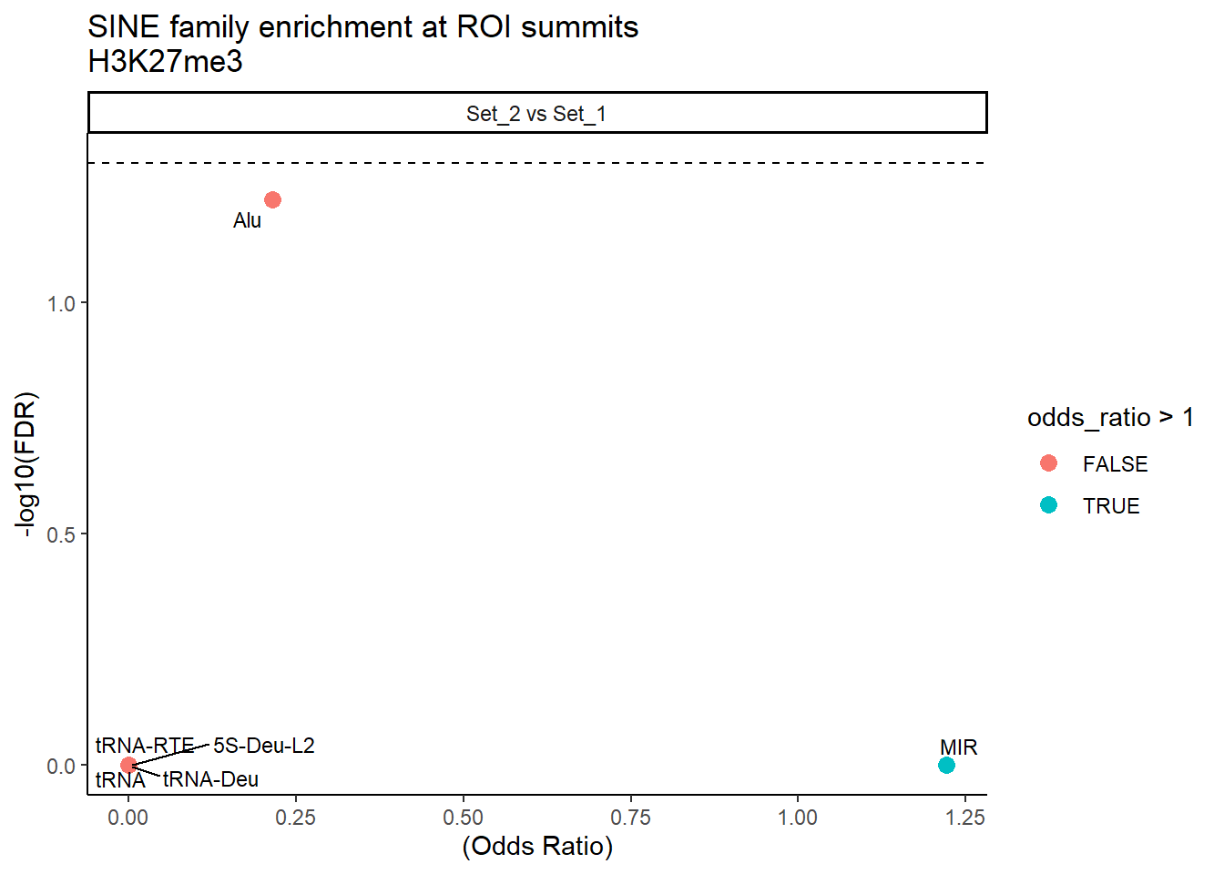
Overlapping SINE family with ROIs to get a count
count_sine_families <- function(peak_gr, sine_gr, cluster_name) {

  hits <- findOverlaps(peak_gr, sine_gr)

  if (length(hits) == 0) {
    return(tibble(
      cluster = cluster_name,
      TE_type = character(),
      status  = character(),
      count   = integer()
    ))
  }

  hit_df <- tibble(
    family = ifelse(
      mcols(sine_gr)$repFamily[subjectHits(hits)] == "SVA",
      mcols(sine_gr)$repName[subjectHits(hits)],
      mcols(sine_gr)$repFamily[subjectHits(hits)]
    )
  )

  ## TE counts per family (Alu/MIR vs SVA_A/B/C…)
  te_counts <- hit_df %>%
    count(family, name = "count") %>%
    mutate(
      cluster = cluster_name,
      TE_type = family,
      status  = "TE"
    )

  ## non-TE peaks (no SINE overlap)
  n_total_peaks <- length(peak_gr)
  n_sine_peaks  <- length(unique(queryHits(hits)))

  not_te <- tibble(
    cluster = cluster_name,
    TE_type = unique(te_counts$TE_type),
    status  = "not_TE",
    count   = n_total_peaks - n_sine_peaks
  )

  bind_rows(te_counts, not_te)
}
fullROI_long_sine <- purrr::imap_dfr(
H3K27me3_sets_gr,
~count_sine_families(.x, SINE_gr, .y)
)
SINE_results_full <- comparisons %>%
mutate(results = map2(cluster2, cluster1, function(c2, c1) {
fullROI_long_sine %>%
distinct(family) %>%
pull() %>%
map_dfr(function(te) {
test_pair_TE_generic(
fullROI_long_sine,
te_name = te,
cluster1 = c1,
cluster2 = c2
)
})
})
) %>%
unnest(results) %>%
mutate(FDR = p.adjust(p_value, method = "BH"))
ggplot(SINE_results_full, aes(x = (odds_ratio), y = -log10(FDR),label = TE_type)) +
geom_point(aes(color = odds_ratio > 1), size = 3) +
# geom_text_repel(data = subset(SVA_results, FDR < 0.05)) +
geom_text_repel(size=3, max.overlaps = Inf)+
geom_hline(yintercept = -log10(0.05), linetype = "dashed") +
geom_vline(xintercept = 1, linetype = 3) +
labs(
x = "(Odds Ratio)",
y = "-log10(FDR)",
title = "SINE family enrichment at full ROI\nH3K27me3"
) +
theme_classic() +
facet_wrap(~comparison)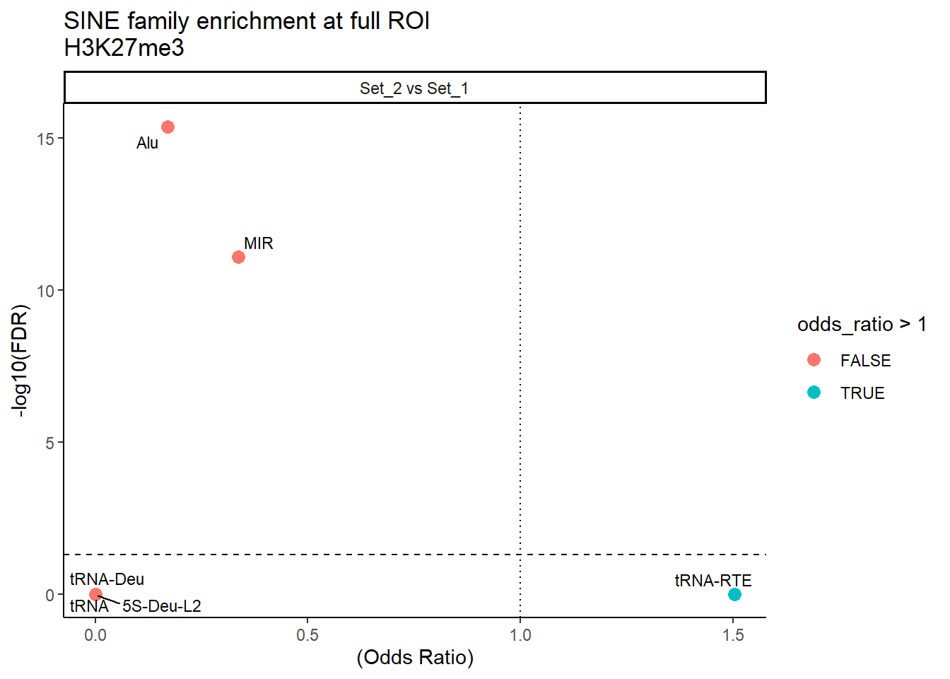
| Version | Author | Date |
|---|---|---|
| ba7cf29 | reneeisnowhere | 2026-01-27 |
LINE
Overlapping LINE family with summits to get a count
LINE_hits <- findOverlaps(H3K27me3_summit_gr, LINE_gr, ignore.strand = TRUE)
LINE_overlap_df <- tibble(
  summit_id = queryHits(LINE_hits),
  cluster   = mcols(H3K27me3_summit_gr)$cluster[queryHits(LINE_hits)],
  TE_type   = mcols(LINE_gr)$repFamily[subjectHits(LINE_hits)])

LINE_counts <- LINE_overlap_df %>%
  count(cluster, TE_type, name = "count") %>%
  mutate(status = "TE")

total_LINE_summits <- tibble(
  cluster = mcols(H3K27me3_summit_gr)$cluster
) %>% count(cluster, name = "total")

not_LINE_counts <- LINE_counts %>%
  left_join(total_LINE_summits, by = "cluster") %>%
  mutate(count = total - count,
         status = "not_TE") %>%
  select(cluster, TE_type, status, count)

LINE_df_long <- bind_rows(LINE_counts %>%
                            dplyr::select(cluster, TE_type, status, count),
                          not_LINE_counts) %>%
  filter(!is.na(cluster))

LINE_results <- comparisons %>%
  mutate(results = map2(cluster2, cluster1, function(c2, c1) {

      LINE_df_long %>%
        distinct(TE_type) %>%
        pull() %>%
        map_dfr(function(te) {
          test_pair_TE_generic(
            LINE_df_long,
            te_name  = te,
            cluster1 = c1,
            cluster2 = c2
          )
        })

    })
  ) %>%
  unnest(results) %>%
  mutate(FDR = p.adjust(p_value, method = "BH"))
datatable(LINE_counts,
rownames = FALSE,
filter = 'top', # add filter/search boxes
options = list(
pageLength = 10,
autoWidth = TRUE,
scrollX = TRUE))total_LINE_summits# A tibble: 3 × 2
cluster total
<chr> <int>
1 Set_1 148910
2 Set_2 235
3 all_H3K27me3_regions 150463# ---- Prepare the table ----
LINE_counts_display <- LINE_results %>%
# 1. Split comparison
separate(comparison, into = c("cluster2", "cluster1"), sep = " vs ", remove = FALSE) %>%
# 2. Add log2 odds ratio
mutate(log2OR = log2(odds_ratio)) %>%
# 3. Add enrichment/depletion direction
mutate(direction = case_when(
odds_ratio > 1 ~ "enriched",
odds_ratio < 1 ~ "depleted",
TRUE ~ "neutral"
)) %>%
# 4. Flag significant
mutate(significant = FDR < 0.05) %>%
# Optional: arrange for readability
arrange(cluster2, direction, desc(log2OR))
# ---- Create interactive datatable ----
datatable(
LINE_counts_display,
rownames = FALSE,
filter = 'top', # add filter/search boxes
options = list(
pageLength = 10,
autoWidth = TRUE,
scrollX = TRUE
)
) %>%
# Conditional coloring by direction
formatStyle(
'direction',
target = 'row',
backgroundColor = styleEqual(
c('enriched', 'depleted'),
c('#FFDD99', '#99CCFF') # enriched = light orange, depleted = light blue
)
) %>%
# Bold significant rows
formatStyle(
'significant',
fontWeight = styleEqual(TRUE, 'bold')
) %>%
# Round numeric columns for readability
formatRound(columns = c('odds_ratio','log2OR','FDR'), digits = 2)ggplot(LINE_results, aes(x = (odds_ratio), y = -log10(FDR),label = TE_type)) +
geom_point(aes(color = odds_ratio > 1), size = 3) +
# geom_text_repel(data = subset(SVA_results, FDR < 0.05)) +
geom_text_repel(size=3, max.overlaps = Inf)+
geom_hline(yintercept = -log10(0.05), linetype = "dashed") +
labs(
x = "(Odds Ratio)",
y = "-log10(FDR)",
title = "LINE family enrichment at ROI summits\nH3K27me3"
) +
theme_classic()+
facet_wrap(~comparison)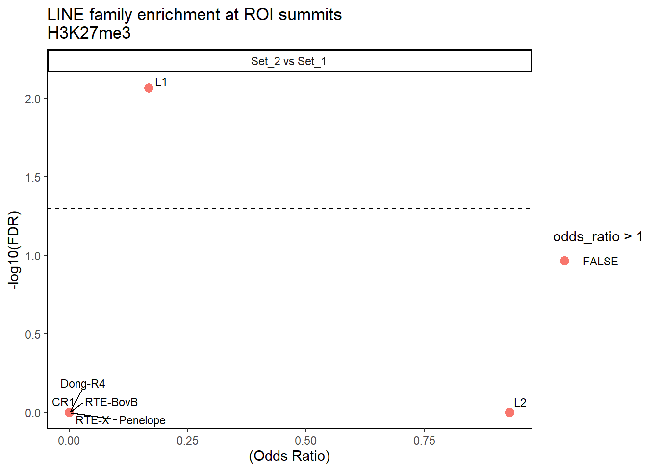
Overlapping LINE family with ROIs to get a count
fullROI_long_LINE <- purrr::imap_dfr(
  H3K27me3_sets_gr,
  ~count_sine_families(.x, LINE_gr, .y)
)


LINE_results_full <- comparisons %>%
  mutate(results = map2(cluster2, cluster1, function(c2, c1) {

      fullROI_long_LINE %>%
        distinct(family) %>%
        pull() %>%
        map_dfr(function(te) {
          test_pair_TE_generic(
            fullROI_long_LINE,
            te_name  = te,
            cluster1 = c1,
            cluster2 = c2
          )
        })

    })
  ) %>%
  unnest(results) %>%
  mutate(FDR = p.adjust(p_value, method = "BH"))

ggplot(LINE_results_full, aes(x = (odds_ratio), y = -log10(FDR),label = TE_type)) +
  geom_point(aes(color = odds_ratio > 1), size = 3) +
   # geom_text_repel(data = subset(SVA_results, FDR < 0.05)) +
  geom_text_repel(size=3, max.overlaps = Inf)+
  geom_hline(yintercept = -log10(0.05), linetype = "dashed") +
    geom_vline(xintercept = 1, linetype = 3) +
  labs(
    x = "(Odds Ratio)",
    y = "-log10(FDR)",
    title = "LINE family enrichment at full ROI\nH3K27me3"
  ) +
  theme_classic() +
  facet_wrap(~comparison)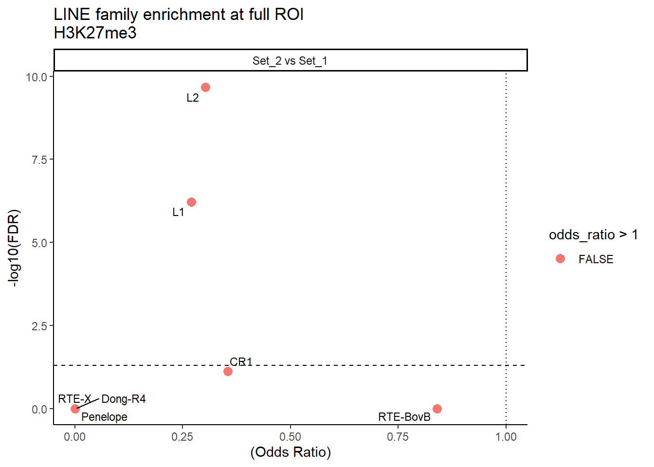
| Version | Author | Date |
|---|---|---|
| ba7cf29 | reneeisnowhere | 2026-01-27 |
LTR
Overlapping LTR family summits to get a count
LTR_hits <- findOverlaps(H3K27me3_summit_gr, LTR_gr, ignore.strand = TRUE)
LTR_overlap_df <- tibble(
  summit_id = queryHits(LTR_hits),
  cluster   = mcols(H3K27me3_summit_gr)$cluster[queryHits(LTR_hits)],
  TE_type   = mcols(LTR_gr)$repFamily[subjectHits(LTR_hits)])

LTR_counts <- LTR_overlap_df %>%
  count(cluster, TE_type, name = "count") %>%
  mutate(status = "TE")

total_LTR_summits <- tibble(
  cluster = mcols(H3K27me3_summit_gr)$cluster
) %>% count(cluster, name = "total")

not_LTR_counts <- LTR_counts %>%
  left_join(total_LTR_summits, by = "cluster") %>%
  mutate(count = total - count,
         status = "not_TE") %>%
  select(cluster, TE_type, status, count)

LTR_df_long <- bind_rows(LTR_counts %>%
                            dplyr::select(cluster, TE_type, status, count),
                          not_LTR_counts) %>%
  filter(!is.na(cluster))

LTR_results <- comparisons %>%
  mutate(results = map2(cluster2, cluster1, function(c2, c1) {

      LTR_df_long %>%
        distinct(TE_type) %>%
        pull() %>%
        map_dfr(function(te) {
          test_pair_TE_generic(
            LTR_df_long,
            te_name  = te,
            cluster1 = c1,
            cluster2 = c2
          )
        })

    })
  ) %>%
  unnest(results) %>%
  mutate(FDR = p.adjust(p_value, method = "BH"))
datatable(LTR_counts,
rownames = FALSE,
filter = 'top', # add filter/search boxes
options = list(
pageLength = 10,
autoWidth = TRUE,
scrollX = TRUE))total_LTR_summits# A tibble: 3 × 2
cluster total
<chr> <int>
1 Set_1 148910
2 Set_2 235
3 all_H3K27me3_regions 150463# ---- Prepare the table ----
LTR_counts_display <- LTR_results %>%
# 1. Split comparison
separate(comparison, into = c("cluster2", "cluster1"), sep = " vs ", remove = FALSE) %>%
# 2. Add log2 odds ratio
mutate(log2OR = log2(odds_ratio)) %>%
# 3. Add enrichment/depletion direction
mutate(direction = case_when(
odds_ratio > 1 ~ "enriched",
odds_ratio < 1 ~ "depleted",
TRUE ~ "neutral"
)) %>%
# 4. Flag significant
mutate(significant = FDR < 0.05) %>%
# Optional: arrange for readability
arrange(cluster2, direction, desc(log2OR))
# ---- Create interactive datatable ----
datatable(
LTR_counts_display,
rownames = FALSE,
filter = 'top', # add filter/search boxes
options = list(
pageLength = 10,
autoWidth = TRUE,
scrollX = TRUE
)
) %>%
# Conditional coloring by direction
formatStyle(
'direction',
target = 'row',
backgroundColor = styleEqual(
c('enriched', 'depleted'),
c('#FFDD99', '#99CCFF') # enriched = light orange, depleted = light blue
)
) %>%
# Bold significant rows
formatStyle(
'significant',
fontWeight = styleEqual(TRUE, 'bold')
) %>%
# Round numeric columns for readability
formatRound(columns = c('odds_ratio','log2OR','FDR'), digits = 2)ggplot(LTR_results, aes(x = (odds_ratio), y = -log10(FDR),label = TE_type)) +
geom_point(aes(color = odds_ratio > 1), size = 3) +
# geom_text_repel(data = subset(SVA_results, FDR < 0.05)) +
geom_text_repel(size=3, max.overlaps = Inf)+
geom_hline(yintercept = -log10(0.05), linetype = "dashed") +
labs(
x = "(Odds Ratio)",
y = "-log10(FDR)",
title = "LTR family enrichment at ROI summits\nH3K27me3"
) +
theme_classic()+
facet_wrap(~comparison)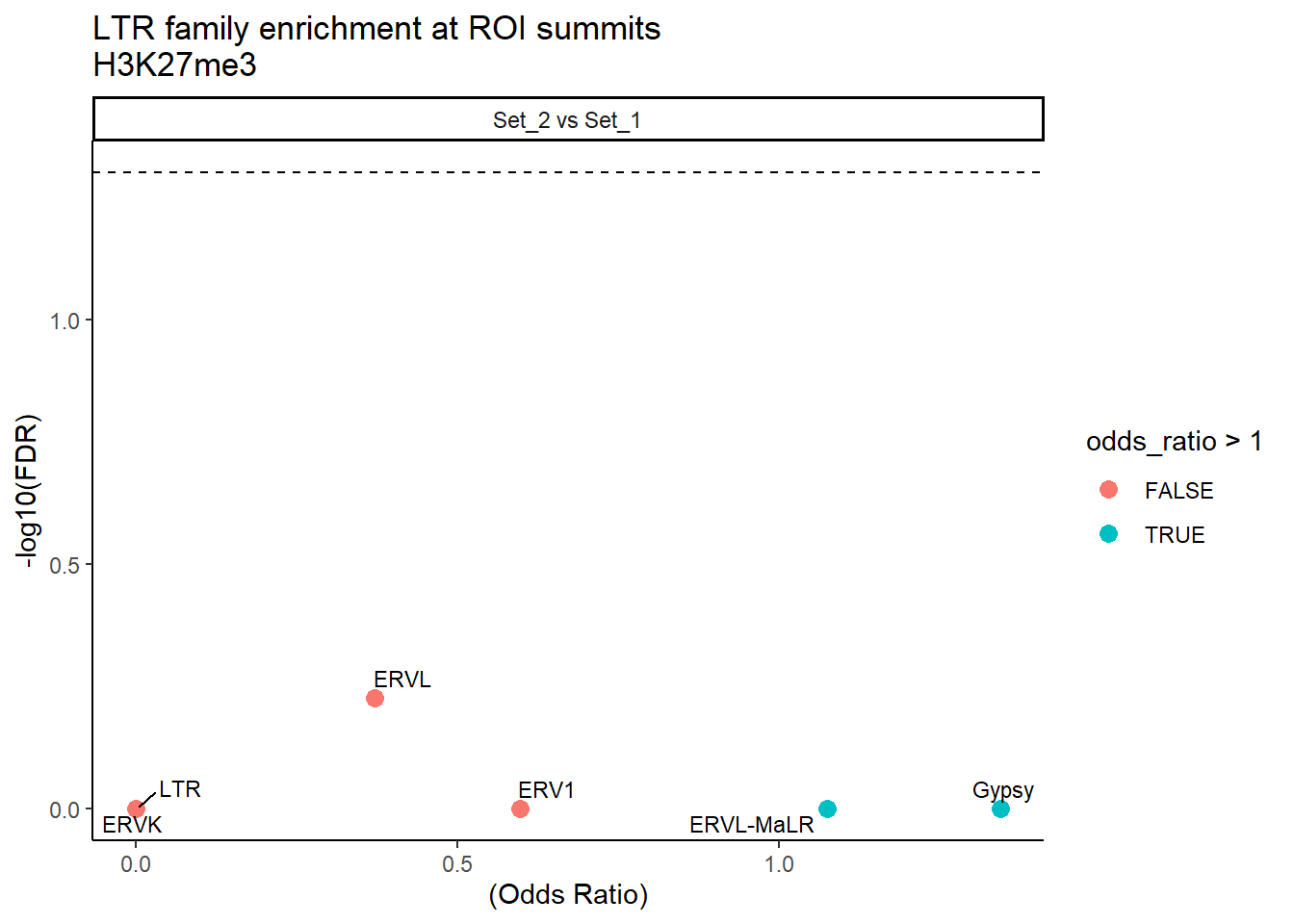
LTR_hits <- findOverlaps(H3K27me3_summit_gr, LTR_gr, ignore.strand = TRUE)
LTR_name_overlap_df <- tibble(
  summit_id = queryHits(LTR_hits),
  cluster   = mcols(H3K27me3_summit_gr)$cluster[queryHits(LTR_hits)],
  TE_type   = mcols(LTR_gr)$repFamily[subjectHits(LTR_hits)],
  repName= mcols(LTR_gr)$repName[subjectHits(LTR_hits)])

LTR_ERV1_counts <-
  LTR_name_overlap_df %>%
    dplyr::filter(TE_type=="ERV1") %>%
  count(cluster, repName, name = "count") %>%
  mutate(status = "TE")

total_LTR_summits <- tibble(
  cluster = mcols(H3K27me3_summit_gr)$cluster
) %>% count(cluster, name = "total")

not_LTR_ERV1_counts <- LTR_ERV1_counts %>%
  left_join(total_LTR_summits, by = "cluster") %>%
  mutate(count = total - count,
         status = "not_TE") %>%
  select(cluster, repName, status, count)

LTR_ERV1_df_long <- bind_rows(LTR_ERV1_counts %>%
                            dplyr::select(cluster, repName, status, count),
                          not_LTR_ERV1_counts) %>%
  filter(!is.na(cluster))

ERV1_LTR_results <- comparisons %>%
  mutate(results = map2(cluster2, cluster1, function(c2, c1) {

       LTR_ERV1_df_long %>%
        distinct(repName) %>%
        pull() %>%
        map_dfr(function(rep) {
          test_pair_TE_repName(
            LTR_ERV1_df_long,
            rep_name  = rep,
            cluster1 = c1,
            cluster2 = c2
          )
        })

    })
  ) %>%
  unnest(results) %>%
  mutate(FDR = p.adjust(p_value, method = "BH"))
ggplot(ERV1_LTR_results, aes(x = (odds_ratio), y = -log10(FDR),label = repName)) +
geom_point(aes(color = odds_ratio > 1), size = 3) +
# geom_text_repel(data = subset(SVA_results, FDR < 0.05)) +
geom_text_repel(data = subset(ERV1_LTR_results, FDR < 0.05), # only significant points
size = 3,
max.overlaps = 100
) +
geom_hline(yintercept = -log10(0.05), linetype = "dashed") +
labs(
x = "(Odds Ratio)",
y = "-log10(FDR)",
title = "LTR Name (type) enrichment at ROI summits\nH3K27me3"
) +
theme_classic()+
facet_wrap(~comparison)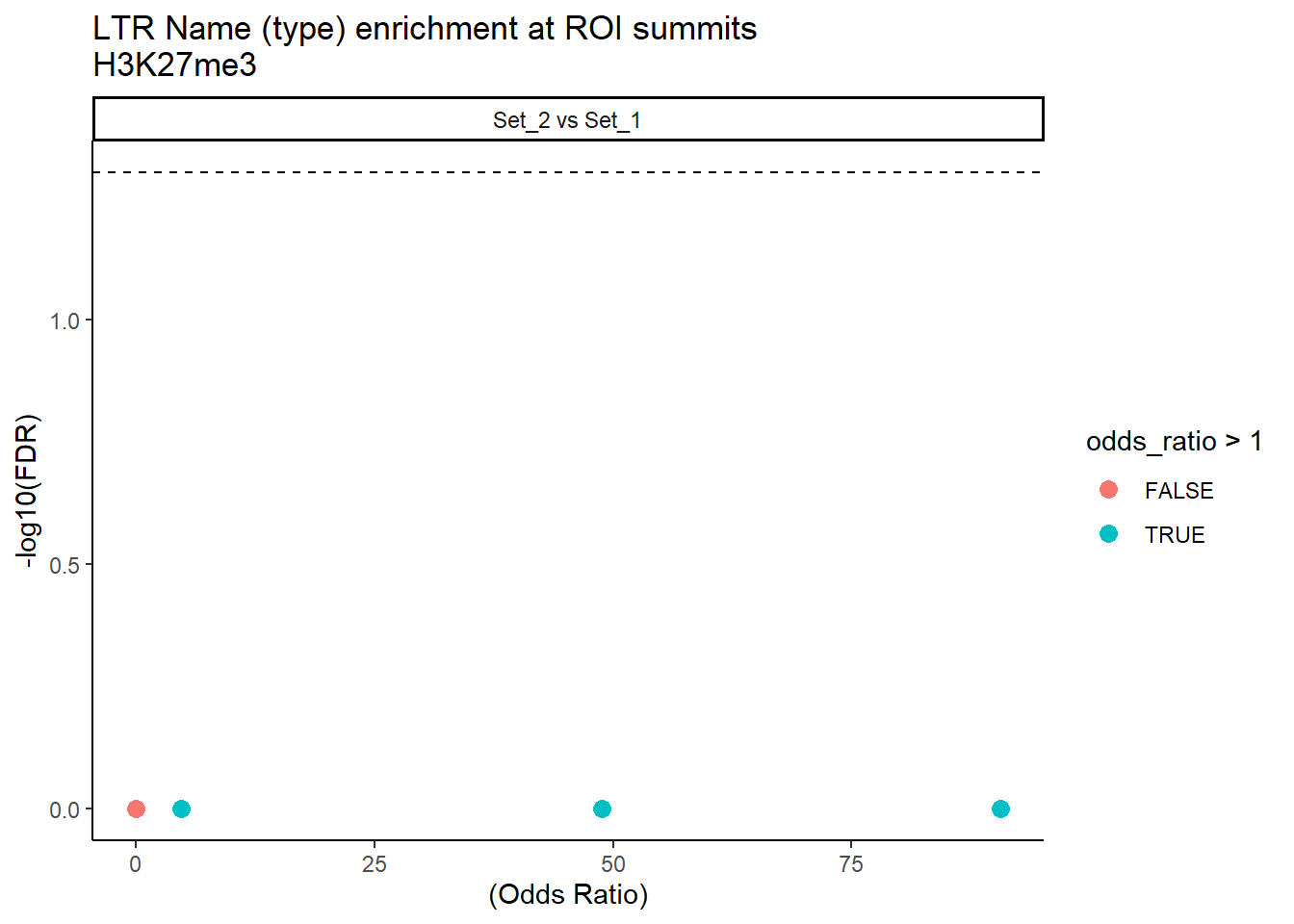
Overlapping LTR family with ROIs to get a count
fullROI_long_LTR <- purrr::imap_dfr(
  H3K27me3_sets_gr,
  ~count_sine_families(.x, LTR_gr, .y)
)


LTR_results_full <- comparisons %>%
  mutate(results = map2(cluster2, cluster1, function(c2, c1) {

      fullROI_long_LTR %>%
        distinct(family) %>%
        pull() %>%
        map_dfr(function(te) {
          test_pair_TE_generic(
            fullROI_long_LTR,
            te_name  = te,
            cluster1 = c1,
            cluster2 = c2
          )
        })

    })
  ) %>%
  unnest(results) %>%
  mutate(FDR = p.adjust(p_value, method = "BH"))

ggplot(LTR_results_full, aes(x = (odds_ratio), y = -log10(FDR),label = TE_type)) +
  geom_point(aes(color = odds_ratio > 1), size = 3) +
   # geom_text_repel(data = subset(SVA_results, FDR < 0.05)) +
  geom_text_repel(size=3, max.overlaps = Inf)+
  geom_hline(yintercept = -log10(0.05), linetype = "dashed") +
    geom_vline(xintercept = 1, linetype = 3) +
  labs(
    x = "(Odds Ratio)",
    y = "-log10(FDR)",
    title = "LTR family enrichment at full ROI\nH3K27me3"
  ) +
  theme_classic() +
  facet_wrap(~comparison)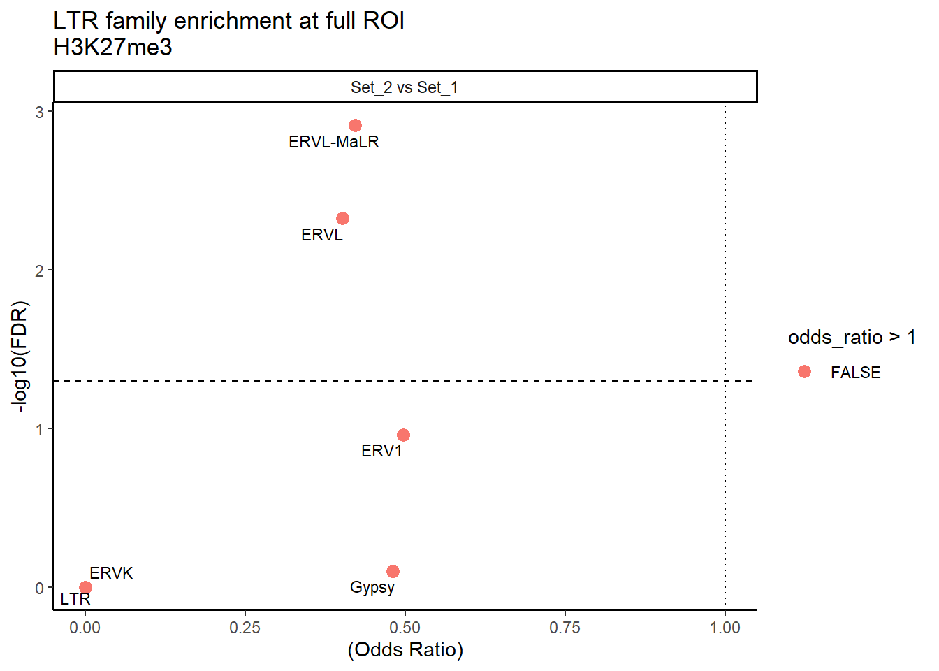
| Version | Author | Date |
|---|---|---|
| ba7cf29 | reneeisnowhere | 2026-01-27 |
SVA
Overlapping SVA family with summits to get a count
SVA_hits <- findOverlaps(H3K27me3_summit_gr, SVA_gr, ignore.strand = TRUE)
SVA_overlap_df <- tibble(
  summit_id = queryHits(SVA_hits),
  cluster   = mcols(H3K27me3_summit_gr)$cluster[queryHits(SVA_hits)],
  TE_type   = mcols(SVA_gr)$repName[subjectHits(SVA_hits)])

SVA_counts <- SVA_overlap_df %>%
  count(cluster, TE_type, name = "count") %>%
  mutate(status = "TE")

total_SVA_summits <- tibble(
  cluster = mcols(H3K27me3_summit_gr)$cluster
) %>% count(cluster, name = "total")

not_SVA_counts <- SVA_counts %>%
  left_join(total_SVA_summits, by = "cluster") %>%
  mutate(count = total - count,
         status = "not_TE") %>%
  select(cluster, TE_type, status, count)

SVA_df_long <- bind_rows(SVA_counts %>%
                            dplyr::select(cluster, TE_type, status, count),
                          not_SVA_counts) %>%
  filter(!is.na(cluster))

SVA_results <- comparisons %>%
  mutate(results = map2(cluster2, cluster1, function(c2, c1) {

      SVA_df_long %>%
        distinct(TE_type) %>%
        pull() %>%
        map_dfr(function(te) {
          test_pair_TE_generic(
            SVA_df_long,
            te_name  = te,
            cluster1 = c1,
            cluster2 = c2
          )
        })

    })
  ) %>%
  unnest(results) %>%
  mutate(FDR = p.adjust(p_value, method = "BH"))
datatable(SVA_counts,
rownames = FALSE,
filter = 'top', # add filter/search boxes
options = list(
pageLength = 10,
autoWidth = TRUE,
scrollX = TRUE))total_SVA_summits# A tibble: 3 × 2
cluster total
<chr> <int>
1 Set_1 148910
2 Set_2 235
3 all_H3K27me3_regions 150463# ---- Prepare the table ----
SVA_counts_display <- SVA_results %>%
# 1. Split comparison
separate(comparison, into = c("cluster2", "cluster1"), sep = " vs ", remove = FALSE) %>%
# 2. Add log2 odds ratio
mutate(log2OR = log2(odds_ratio)) %>%
# 3. Add enrichment/depletion direction
mutate(direction = case_when(
odds_ratio > 1 ~ "enriched",
odds_ratio < 1 ~ "depleted",
TRUE ~ "neutral"
)) %>%
# 4. Flag significant
mutate(significant = FDR < 0.05) %>%
# Optional: arrange for readability
arrange(cluster2, direction, desc(log2OR))
# ---- Create interactive datatable ----
datatable(
SVA_counts_display,
rownames = FALSE,
filter = 'top', # add filter/search boxes
options = list(
pageLength = 10,
autoWidth = TRUE,
scrollX = TRUE
)
) %>%
# Conditional coloring by direction
formatStyle(
'direction',
target = 'row',
backgroundColor = styleEqual(
c('enriched', 'depleted'),
c('#FFDD99', '#99CCFF') # enriched = light orange, depleted = light blue
)
) %>%
# Bold significant rows
formatStyle(
'significant',
fontWeight = styleEqual(TRUE, 'bold')
) %>%
# Round numeric columns for readability
formatRound(columns = c('odds_ratio','log2OR','FDR'), digits = 2)ggplot(SVA_results, aes(x = (odds_ratio), y = -log10(FDR),label = TE_type)) +
geom_point(aes(color = odds_ratio > 1), size = 3) +
# geom_text_repel(data = subset(SVA_results, FDR < 0.05)) +
geom_text_repel(size=3, max.overlaps = Inf)+
geom_hline(yintercept = -log10(0.05), linetype = "dashed") +
labs(
x = "(Odds Ratio)",
y = "-log10(FDR)",
title = "SVA family enrichment at ROI summits\nH3K27me3"
) +
theme_classic()+
facet_wrap(~comparison)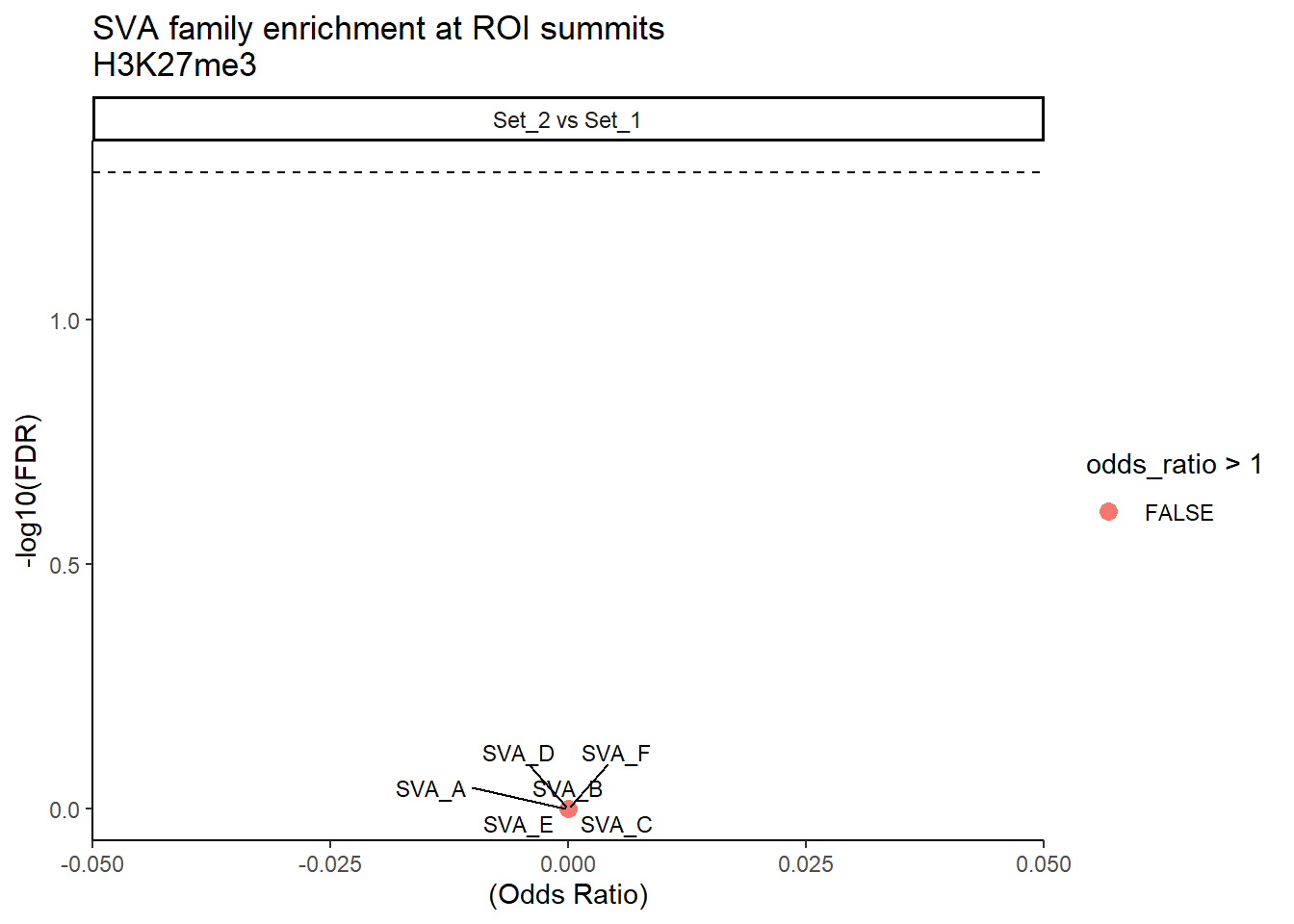
Overlapping SVA family with ROIs to get a count
fullROI_long_SVA <- purrr::imap_dfr(
  H3K27me3_sets_gr,
  ~count_sine_families(.x, SVA_gr, .y)
)


SVA_results_full <- comparisons %>%
  mutate(results = map2(cluster2, cluster1, function(c2, c1) {

      fullROI_long_SVA %>%
        distinct(family) %>%
        pull() %>%
        map_dfr(function(te) {
          test_pair_TE_generic(
            fullROI_long_SVA,
            te_name  = te,
            cluster1 = c1,
            cluster2 = c2
          )
        })

    })
  ) %>%
  unnest(results) %>%
  mutate(FDR = p.adjust(p_value, method = "BH"))

ggplot(SVA_results_full, aes(x = (odds_ratio), y = -log10(FDR),label = TE_type)) +
  geom_point(aes(color = odds_ratio > 1), size = 3) +
   # geom_text_repel(data = subset(SVA_results, FDR < 0.05)) +
  geom_text_repel(size=3, max.overlaps = Inf)+
  geom_hline(yintercept = -log10(0.05), linetype = "dashed") +
    geom_vline(xintercept = 1, linetype = 3) +
  labs(
    x = "(Odds Ratio)",
    y = "-log10(FDR)",
    title = "SVA family enrichment at full ROI\nH3K27me3"
  ) +
  theme_classic() +
  facet_wrap(~comparison)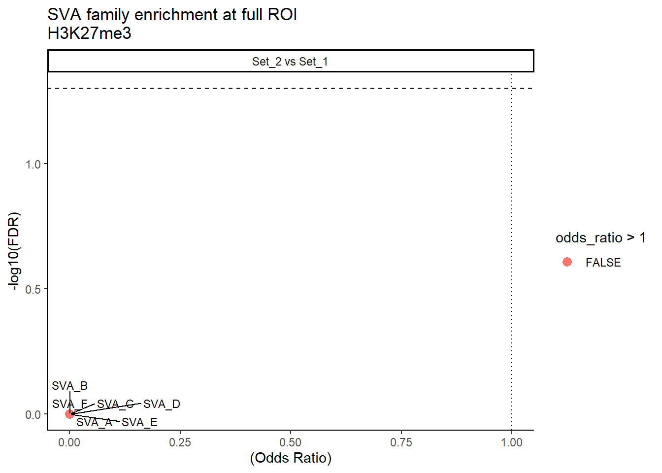
| Version | Author | Date |
|---|---|---|
| ba7cf29 | reneeisnowhere | 2026-01-27 |
DNA
Overlapping DNA family with summits to get a count
DNA_hits <- findOverlaps(H3K27me3_summit_gr, DNA_gr, ignore.strand = TRUE)
DNA_overlap_df <- tibble(
  summit_id = queryHits(DNA_hits),
  cluster   = mcols(H3K27me3_summit_gr)$cluster[queryHits(DNA_hits)],
  TE_type   = mcols(DNA_gr)$repFamily[subjectHits(DNA_hits)])

DNA_counts <- DNA_overlap_df %>%
  count(cluster, TE_type, name = "count") %>%
  mutate(status = "TE")

total_DNA_summits <- tibble(
  cluster = mcols(H3K27me3_summit_gr)$cluster
) %>% count(cluster, name = "total")

not_DNA_counts <- DNA_counts %>%
  left_join(total_DNA_summits, by = "cluster") %>%
  mutate(count = total - count,
         status = "not_TE") %>%
  select(cluster, TE_type, status, count)

DNA_df_long <- bind_rows(DNA_counts %>%
                            dplyr::select(cluster, TE_type, status, count),
                          not_DNA_counts) %>%
  filter(!is.na(cluster))

DNA_results <- comparisons %>%
  mutate(results = map2(cluster2, cluster1, function(c2, c1) {

      DNA_df_long %>%
        distinct(TE_type) %>%
        pull() %>%
        map_dfr(function(te) {
          test_pair_TE_generic(
            DNA_df_long,
            te_name  = te,
            cluster1 = c1,
            cluster2 = c2
          )
        })

    })
  ) %>%
  unnest(results) %>%
  mutate(FDR = p.adjust(p_value, method = "BH"))
datatable(DNA_counts,
rownames = FALSE,
filter = 'top', # add filter/search boxes
options = list(
pageLength = 10,
autoWidth = TRUE,
scrollX = TRUE))total_DNA_summits# A tibble: 3 × 2
cluster total
<chr> <int>
1 Set_1 148910
2 Set_2 235
3 all_H3K27me3_regions 150463# ---- Prepare the table ----
DNA_counts_display <- DNA_results %>%
# 1. Split comparison
separate(comparison, into = c("cluster2", "cluster1"), sep = " vs ", remove = FALSE) %>%
# 2. Add log2 odds ratio
mutate(log2OR = log2(odds_ratio)) %>%
# 3. Add enrichment/depletion direction
mutate(direction = case_when(
odds_ratio > 1 ~ "enriched",
odds_ratio < 1 ~ "depleted",
TRUE ~ "neutral"
)) %>%
# 4. Flag significant
mutate(significant = FDR < 0.05) %>%
# Optional: arrange for readability
arrange(cluster2, direction, desc(log2OR))
# ---- Create interactive datatable ----
datatable(
DNA_counts_display,
rownames = FALSE,
filter = 'top', # add filter/search boxes
options = list(
pageLength = 10,
autoWidth = TRUE,
scrollX = TRUE
)
) %>%
# Conditional coloring by direction
formatStyle(
'direction',
target = 'row',
backgroundColor = styleEqual(
c('enriched', 'depleted'),
c('#FFDD99', '#99CCFF') # enriched = light orange, depleted = light blue
)
) %>%
# Bold significant rows
formatStyle(
'significant',
fontWeight = styleEqual(TRUE, 'bold')
) %>%
# Round numeric columns for readability
formatRound(columns = c('odds_ratio','log2OR','FDR'), digits = 2)ggplot(DNA_results, aes(x = (odds_ratio), y = -log10(FDR),label = TE_type)) +
geom_point(aes(color = odds_ratio > 1), size = 3) +
# geom_text_repel(data = subset(SVA_results, FDR < 0.05)) +
geom_text_repel(size=3, max.overlaps = Inf)+
geom_hline(yintercept = -log10(0.05), linetype = "dashed") +
labs(
x = "(Odds Ratio)",
y = "-log10(FDR)",
title = "DNA family enrichment at ROI summits\nH3K27me3"
) +
theme_classic()+
facet_wrap(~comparison)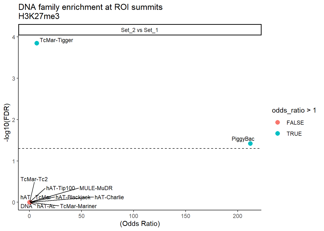
peakAnnoList_H3K27me3 <- readRDS("data/motif_lists/H3K27me3_annotated_peaks.RDS")

out_dir <- "data/Bed_exports/H3K27me3_sets"
set_list <- names(peakAnnoList_H3K27me3)

for (group_name in set_list) {
  cs <- peakAnnoList_H3K27me3[[group_name]]
  gr <- cs@anno

  # Set BED name column
  mcols(gr)$name <- mcols(gr)$Peakid

  # Optional: if you want a score column
  if(!"score" %in% colnames(mcols(gr))) {
    mcols(gr)$score <- 0
  }

  # Export to BED
 bed_file <- file.path(out_dir, paste0(group_name, "_H3K27me3.bed"))

  # Export
  export(gr, bed_file, format = "BED")

  cat("Exported:", bed_file, "\n")
}
Overlapping DNA family with ROIs to get a count
fullROI_long_DNA <- purrr::imap_dfr(
  H3K27me3_sets_gr,
  ~count_sine_families(.x, DNA_gr, .y)
)


DNA_results_full <- comparisons %>%
  mutate(results = map2(cluster2, cluster1, function(c2, c1) {

      fullROI_long_DNA %>%
        distinct(family) %>%
        pull() %>%
        map_dfr(function(te) {
          test_pair_TE_generic(
            fullROI_long_DNA,
            te_name  = te,
            cluster1 = c1,
            cluster2 = c2
          )
        })

    })
  ) %>%
  unnest(results) %>%
  mutate(FDR = p.adjust(p_value, method = "BH"))

ggplot(DNA_results_full, aes(x = (odds_ratio), y = -log10(FDR),label = TE_type)) +
  geom_point(aes(color = odds_ratio > 1), size = 3) +
   # geom_text_repel(data = subset(SVA_results, FDR < 0.05)) +
  geom_text_repel(size=3, max.overlaps = Inf)+
  geom_hline(yintercept = -log10(0.05), linetype = "dashed") +
    geom_vline(xintercept = 1, linetype = 3) +
  labs(
    x = "(Odds Ratio)",
    y = "-log10(FDR)",
    title = "DNA family enrichment at full ROI\nH3K27me3"
  ) +
  theme_classic() +
  facet_wrap(~comparison)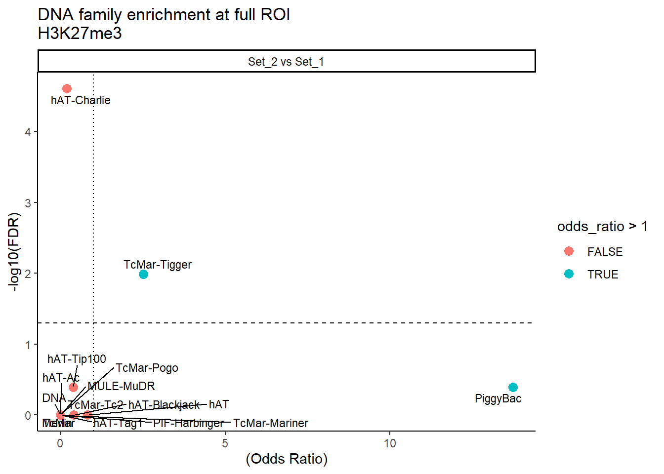
| Version | Author | Date |
|---|---|---|
| ba7cf29 | reneeisnowhere | 2026-01-27 |
Proportions of SETs and SETS of TEs
annotated_tables <- H3K27me3_sets_gr$all_H3K27me3_regions %>% as.data.frame()
anno_H3K27me3_summits <- readRDS("data/TE_annotation/H3K27me3_annotated_summit_TE_overlaps.RDS")
anno_H3K27me3 <- annotated_tables
# H3K27me3_set_case_lookup <- bind_rows(H3K27me3_set_case_lfc, .id = "set_case") %>%
# dplyr::select(Peakid,cluster:set_case)
anno_H3K27me3 %>%
left_join(H3K27me3_lookup) %>%
group_by(cluster) %>%
count() %>%
ungroup() %>%
mutate(percent = n / sum(n)) %>%
ggplot(.,aes(x=cluster, y=percent, fill=cluster)) +
geom_col() +
geom_text(
aes(label = sprintf("%.3f", percent)),
vjust = -0.3,
size = 3
) +
ylab("proportion")+
ggtitle("Proportion of ROIs by cluster, H3K27me3")+
theme_bw() +
theme(
axis.text.x = element_text(angle = 45, hjust = 1),
strip.text = element_text(face = "bold")
)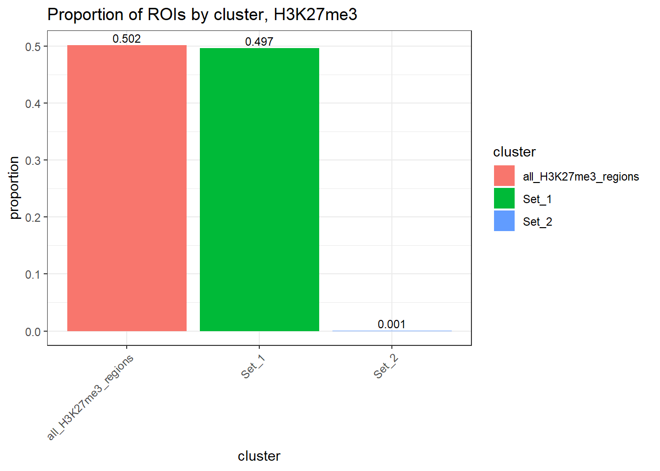 ### TE proportions by ROI-summits
H3K27me3_te_summary_summits <- anno_H3K27me3_summits %>%
left_join(H3K27me3_lookup) %>%
mutate(repClass = na_if(repClass, ""), # treat empty as NA
n_TE_class = case_when(
is.na(repClass) ~ 0L,
TRUE ~ lengths(strsplit(repClass, ";")))) %>%
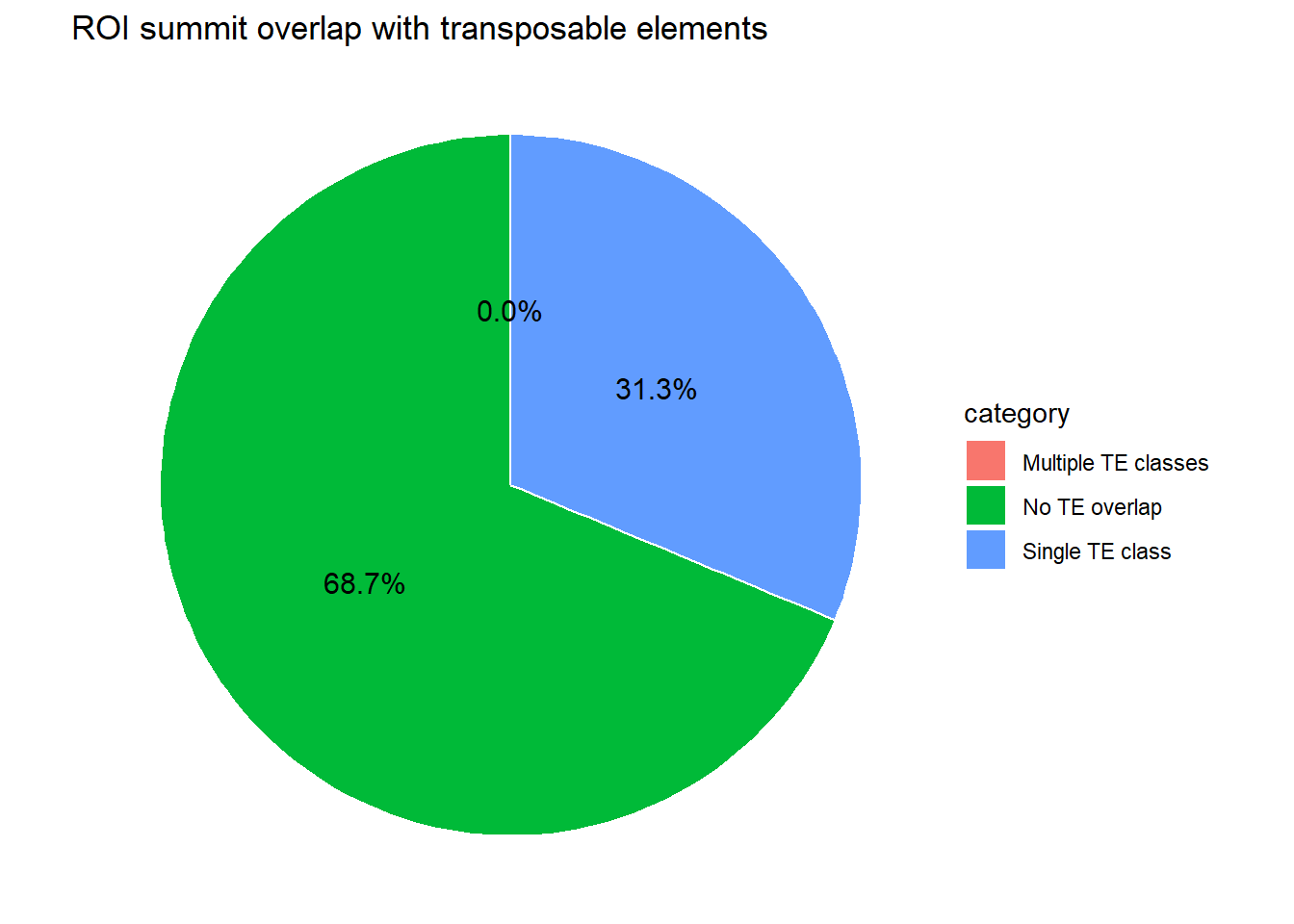
mutate( category = case_when(n_TE_class == 0 ~ "No TE overlap",
n_TE_class == 1 ~ "Single TE class",
n_TE_class > 1 ~ "Multiple TE classes"))
pie_df_summits <- H3K27me3_te_summary_summits %>%
count(category) %>%
mutate(
percent = n / sum(n) * 100
)
ggplot(pie_df_summits, aes(x = "", y = percent, fill = category)) +
geom_col(width = 1, color = "white") +
coord_polar(theta = "y") +
theme_void() +
geom_text(
aes(label = sprintf("%.1f%%", percent)),
position = position_stack(vjust = 0.5),
size = 4
) +
labs(
title = "ROI summit overlap with transposable elements"
)
H3K27me3_te_family_long_summits <- H3K27me3_te_summary_summits %>%
  filter(!is.na(repClass), repClass != "") %>%   # TE-positive only
  separate_rows(repClass, sep = ";") %>%
  distinct(Peakid, repClass,cluster)


fam_pie_df_summits <- H3K27me3_te_family_long_summits %>%
  count(repClass, name = "n") %>%
  mutate(percent = n / sum(n)*100) %>%
  mutate(
    repClass = if_else(percent < 2, "Other", repClass)
  ) %>%
  group_by(repClass) %>%
  summarise(n = sum(n), .groups = "drop") %>%
  mutate(percent = n / sum(n) * 100)


ggplot(fam_pie_df_summits, aes(x = "", y = percent, fill = repClass)) +
  geom_col(width = 1, color = "white") +
  coord_polar(theta = "y") +
  theme_void() +
  geom_text(
    aes(label = sprintf("%s\n%.1f%%", repClass, percent)),
    position = position_stack(vjust = 0.5),
    size = 3
  ) +
  labs(
    title = "TE Class composition among TE-overlapping ROI summits",
    fill = "TE Class")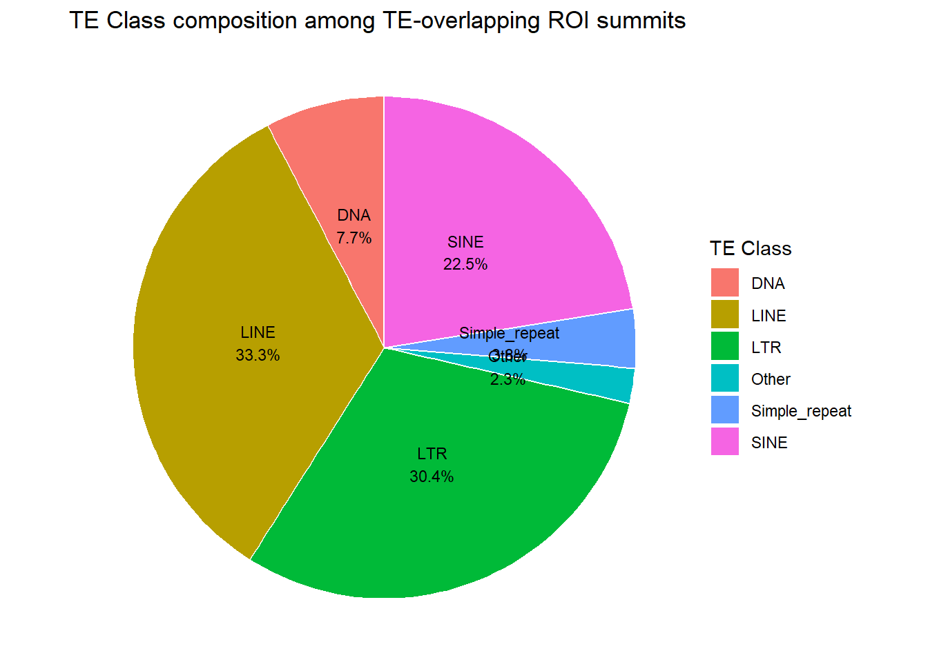
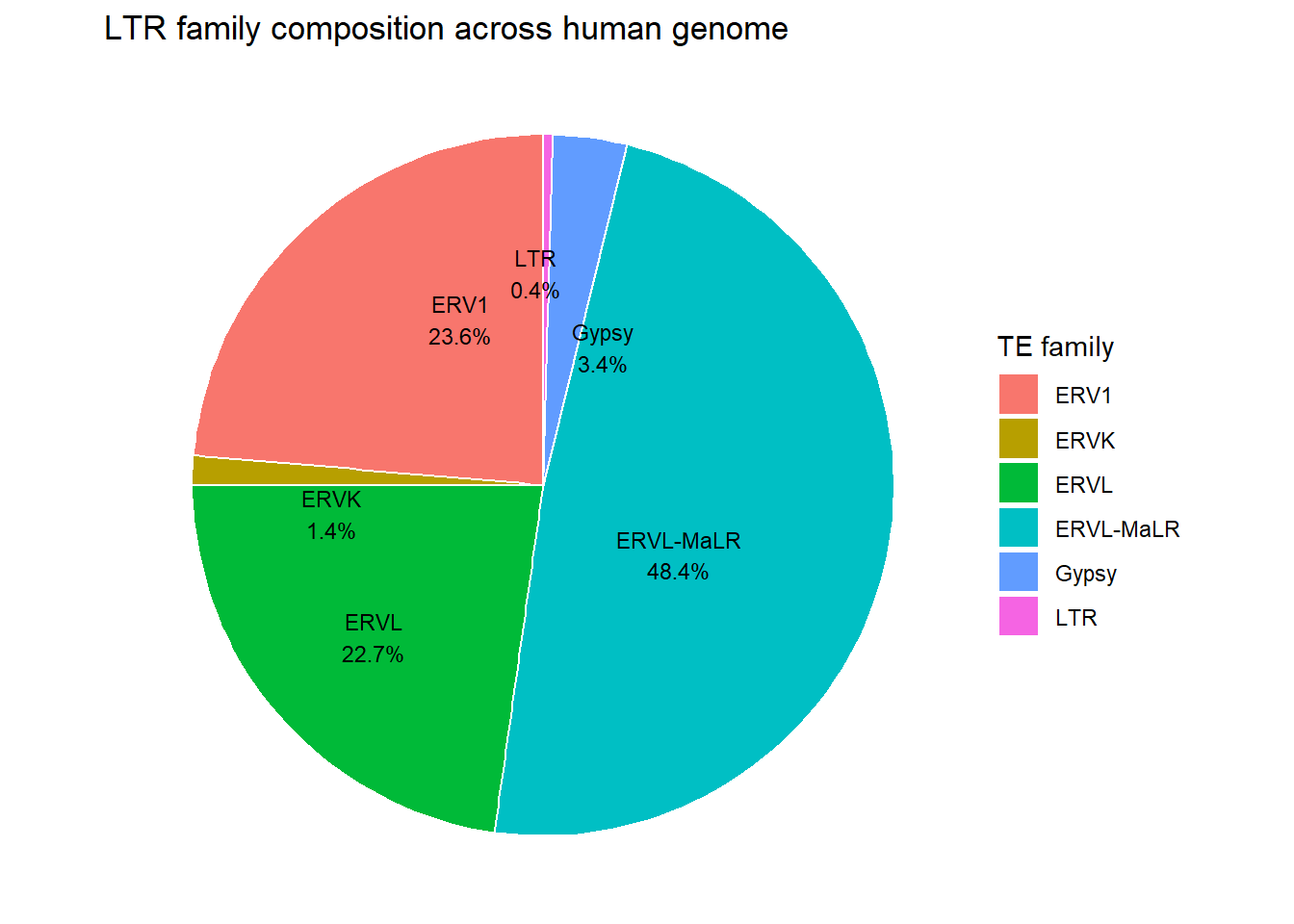
# unique(rpt_split_gr_list$LTR$repFamily)human_genome_LTR <- LTR_df %>%
dplyr::filter(repFamily %in% c("ERV1", "ERVK","ERVL", "ERVL-MaLR","Gypsy","LTR")) %>%
count(repFamily, name = "n") %>%
mutate(percent= n/ sum(n) * 100)
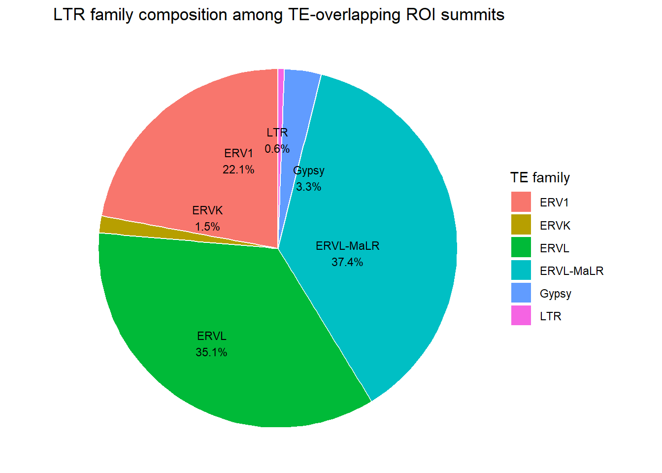
H3K27me3_long_repFamily_summits <- H3K27me3_te_summary_summits %>%
filter(!is.na(repFamily), repFamily != "") %>% # TE-positive only
separate_rows(repFamily, sep = ";") %>%
distinct(Peakid, repFamily)
H3K27me3_LTR_pie_df_summits <- H3K27me3_long_repFamily_summits %>%
dplyr::filter(repFamily %in% c("ERV1", "ERVK","ERVL", "ERVL-MaLR","Gypsy","LTR")) %>%
count(repFamily, name = "n") %>%
mutate(percent= n/ sum(n) * 100)
ggplot(H3K27me3_LTR_pie_df_summits, aes(x = "", y = percent, fill = repFamily)) +
geom_col(width = 1, color = "white") +
coord_polar(theta = "y") +
theme_void() +
geom_text_repel(
aes(label = sprintf("%s\n%.1f%%", repFamily, percent)),
position = position_stack(vjust = 0.5),
size = 3
) +
labs(
title = "LTR family composition among TE-overlapping ROI summits",
fill = "TE family"
)
ggplot(human_genome_LTR, aes(x = "", y = percent, fill = repFamily)) +
  geom_col(width = 1, color = "white") +
  coord_polar(theta = "y") +
  theme_void() +
  geom_text_repel(
    aes(label = sprintf("%s\n%.1f%%", repFamily, percent)),
    position = position_stack(vjust = 0.5),
    size = 3
  ) +
  labs(
    title = "LTR family composition across human genome",
    fill = "TE family"
  )
rpt_genome <- repeatmasker_clean %>%
mutate(cluster = "hg38") %>%
group_by(cluster, repClass) %>%
summarise(n = n(), .groups = "drop") %>%
mutate(percent = n / sum(n) * 100) %>%
mutate(
repClass = if_else(percent < 1.2, "Other", repClass)
) %>%
group_by(repClass) %>%
summarise(n = sum(n), .groups = "drop") %>%
mutate(percent = n / sum(n) * 100)
H3K27me3_te_family_clust_summits <- H3K27me3_te_family_long_summits %>%
dplyr::filter(cluster != "not_assigned") %>%
distinct(Peakid, cluster, repClass) %>%
count(cluster, repClass, name = "n") %>%
group_by(cluster) %>%
mutate(percent = n / sum(n)*100) %>%
mutate(
repClass = if_else(percent < 2, "Other", repClass)
) %>%
group_by(cluster,repClass) %>%
summarise(n = sum(n), .groups = "drop") %>%
group_by(cluster) %>%
mutate(percent = n / sum(n) * 100) %>%
rbind((rpt_genome %>% mutate(cluster="hg38")))
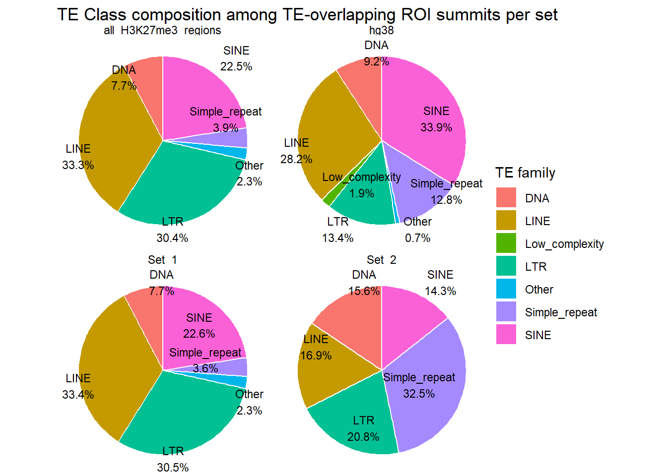
ggplot(H3K27me3_te_family_clust_summits, aes(x = "", y=percent, fill=repClass))+
geom_col(width =1, color="white")+
coord_polar(theta = "y")+
geom_text_repel(
aes(x= 1.5,label = sprintf("%s\n%.1f%%", repClass, percent)),
position = position_stack(vjust = 0.5),
size = 3
) +
facet_wrap(~cluster)+
theme_void()+
labs(
title = "TE Class composition among TE-overlapping ROI summits per set",
fill = "TE family"
)
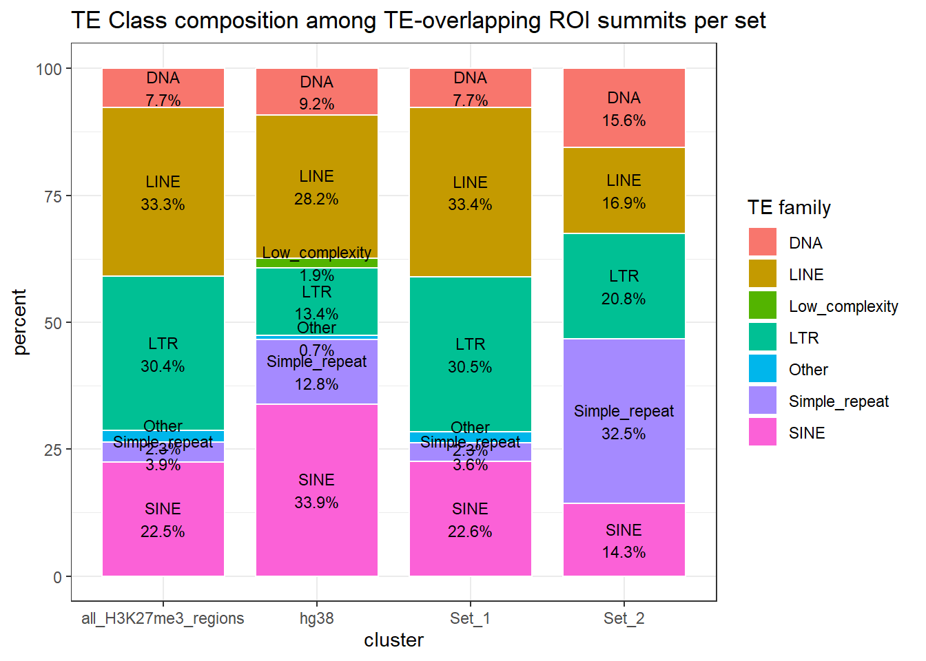
ggplot(H3K27me3_te_family_clust_summits, aes(x = cluster, y=percent, fill=repClass))+
   geom_col(width = 0.8, color = "white") +
  geom_text(
    aes(label = sprintf("%s\n%.1f%%", repClass, percent)),
    position = position_stack(vjust = 0.5),
    size = 3
  ) +
  theme_bw() +
  labs(
    title = "TE Class composition among TE-overlapping ROI summits per set",
    fill = "TE family"
  )
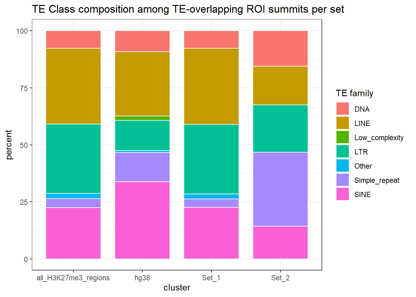
  ggplot(H3K27me3_te_family_clust_summits, aes(x = cluster, y=percent, fill=repClass))+
   geom_col(width = 0.8, color = "white") +
  # geom_text(
  #   aes(label = sprintf("%s\n%.1f%%", repClass, percent)),
  #   position = position_stack(vjust = 0.5),
  #   size = 3
  # ) +
  theme_bw() +
  labs(
    title = "TE Class composition among TE-overlapping ROI summits per set",
    fill = "TE family"
  )
LTR_genome <-
repeatmasker_clean %>%
mutate(cluster = "hg38") %>%
dplyr::filter(repFamily %in% c("ERV1", "ERVK","ERVL", "ERVL-MaLR","Gypsy","LTR"))%>%
group_by(repFamily) %>%
summarise(n = dplyr::n(), .groups = "drop") %>%
mutate(percent = n / sum(n) * 100)
H3K27me3_long_repFamily_summits <-
H3K27me3_te_summary_summits %>%
dplyr::filter(cluster != "not_assigned") %>%
filter(!is.na(repFamily), repFamily != "") %>% # TE-positive only
separate_rows(repFamily, sep = ";") %>%
distinct(cluster,Peakid, repFamily) %>%
dplyr::filter(repFamily %in% c("ERV1", "ERVK","ERVL", "ERVL-MaLR","Gypsy","LTR")) %>%
count(cluster,repFamily, name = "n") %>%
group_by(cluster) %>%
mutate(percent = n / sum(n)*100) %>%
group_by(cluster,repFamily) %>%
summarise(n = sum(n), .groups = "drop") %>%
group_by(cluster) %>%
mutate(percent = n / sum(n) * 100) %>%
rbind((LTR_genome %>% mutate(cluster="hg38")))
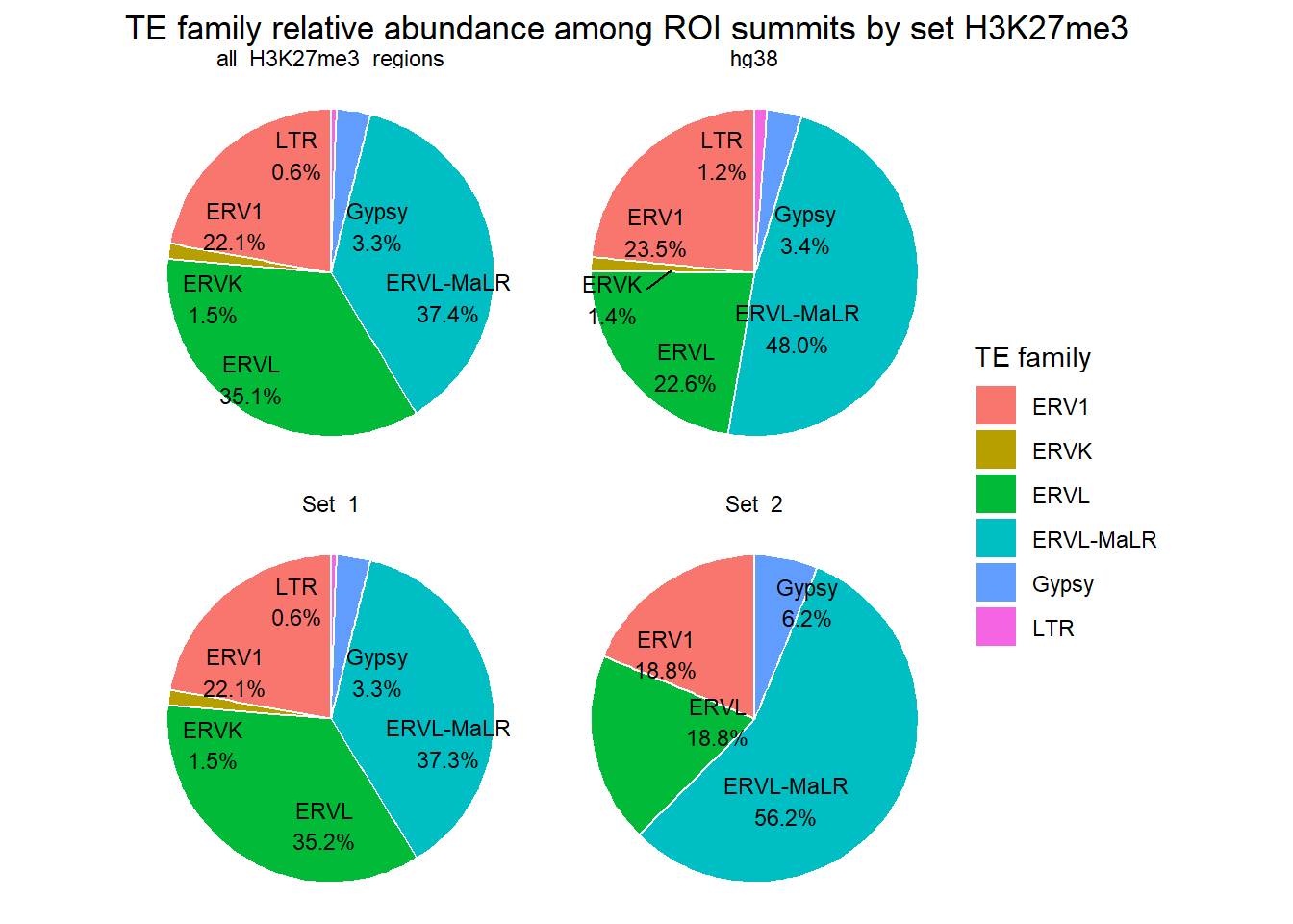
ggplot(H3K27me3_long_repFamily_summits, aes(x = "", y=percent, fill=repFamily))+
geom_col(width =1, color="white")+
coord_polar(theta = "y")+
geom_text_repel(
aes(label = sprintf("%s\n%.1f%%", repFamily, percent)),
position = position_stack(vjust = 0.5),
size = 3,
show.legend = FALSE
) +
facet_wrap(~cluster)+
theme_void()+
labs(
title = "TE family relative abundance among ROI summits by set H3K27me3",
fill = "TE family"
)
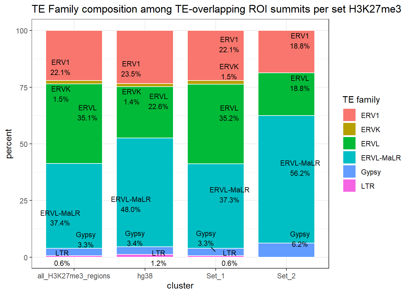
ggplot(H3K27me3_long_repFamily_summits, aes(x = cluster, y=percent, fill=repFamily))+
   geom_col(width = 0.8, color = "white") +
  geom_text_repel(
    aes(label = sprintf("%s\n%.1f%%", repFamily, percent)),
    position = position_stack(vjust = 0.5),
    size = 3
  ) +
  theme_bw() +
  labs(
    title = "TE Family composition among TE-overlapping ROI summits per set H3K27me3",
    fill = "TE family"
  )
LTR_bar_df_summits <-H3K27me3_te_summary_summits %>%
  filter(!is.na(repFamily), repFamily != "")  %>%   # TE-positive only
  separate_rows(repFamily, sep = ";") %>%
  distinct(cluster,Peakid, repFamily) %>%
  dplyr::filter(repFamily %in% c("ERV1", "ERVK","ERVL", "ERVL-MaLR","Gypsy","LTR")) %>%
  group_by(repFamily, cluster) %>%
  summarise(n = dplyr::n(), .groups = "drop") %>%
  # optionally convert NA to a string
  mutate(cluster = if_else(is.na(cluster), "NA", cluster))

ggplot(LTR_bar_df_summits, aes(x = repFamily, y = n, fill = cluster)) +
  geom_col(position = "fill") +
  theme_classic() +
  labs(
    x = "LTR Family",
    y = "Proportion of ROIs",
    fill = "Cluster",
    title = "Proportion of ROI summits across each LTR family"
  ) +
  theme(axis.text.x = element_text(angle = 45, hjust = 1))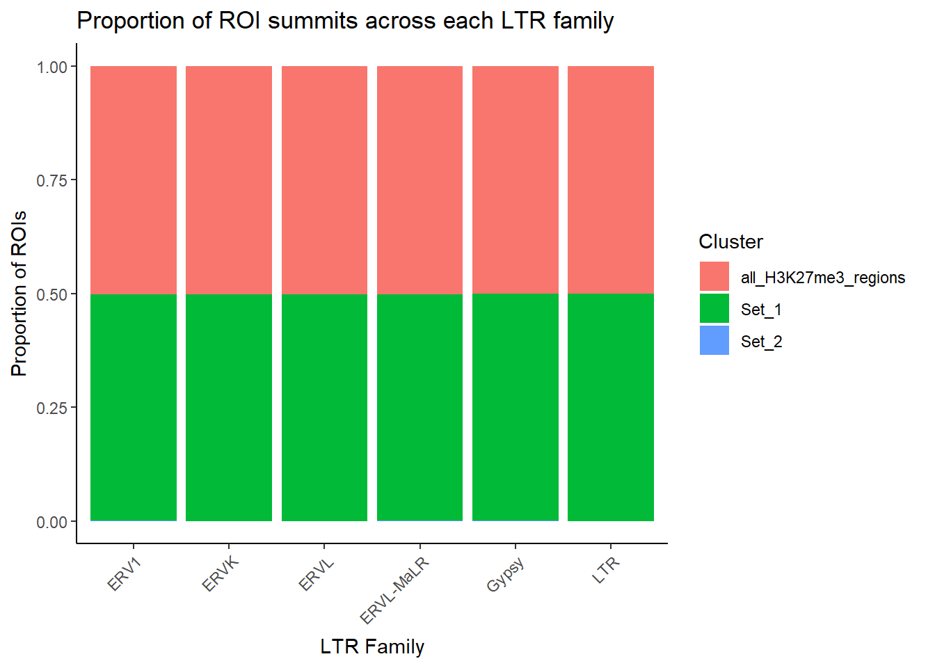
summit_H3K27me3_LTR_breakdown <- anno_H3K27me3_summits %>%
  left_join(H3K27me3_lookup) %>%
   mutate(repClass = na_if(repClass, "")) %>%
  dplyr::filter(repFamily %in% c("ERV1", "ERVK","ERVL", "ERVL-MaLR","Gypsy","LTR")) %>%
  dplyr::select(Peakid, repClass,repFamily, repName, cluster)

summit_H3K27me3_LTR_breakdown %>%
  # dplyr::filter(repFamily=="ERVK") %>%
  group_by(repFamily,cluster) %>% tally() %>%
pivot_wider(., id_cols=repFamily, names_from = cluster, values_from = n)
# A tibble: 6 × 4
# Groups: repFamily [6]
repFamily Set_1 Set_2 all_H3K27me3_regions
<chr> <int> <int> <int>
1 ERV1 3152 3 3170
2 ERVK 218 NA 220
3 ERVL 5009 3 5039
4 ERVL-MaLR 5314 9 5365
5 Gypsy 472 1 474
6 LTR 84 NA 84
sessionInfo()R version 4.4.2 (2024-10-31 ucrt)
Platform: x86_64-w64-mingw32/x64
Running under: Windows 11 x64 (build 26200)
Matrix products: default
locale:
[1] LC_COLLATE=English_United States.utf8
[2] LC_CTYPE=English_United States.utf8
[3] LC_MONETARY=English_United States.utf8
[4] LC_NUMERIC=C
[5] LC_TIME=English_United States.utf8
time zone: America/Chicago
tzcode source: internal
attached base packages:
[1] grid stats4 stats graphics grDevices utils datasets
[8] methods base
other attached packages:
[1] ChIPseeker_1.42.1 DT_0.33 ggrepel_0.9.6
[4] rtracklayer_1.66.0 genomation_1.38.0 plyranges_1.26.0
[7] GenomicRanges_1.58.0 GenomeInfoDb_1.42.3 IRanges_2.40.1
[10] S4Vectors_0.44.0 BiocGenerics_0.52.0 lubridate_1.9.4
[13] forcats_1.0.0 stringr_1.5.1 dplyr_1.1.4
[16] purrr_1.1.0 readr_2.1.5 tidyr_1.3.1
[19] tibble_3.3.0 ggplot2_3.5.2 tidyverse_2.0.0
[22] workflowr_1.7.1
loaded via a namespace (and not attached):
[1] RColorBrewer_1.1-3
[2] rstudioapi_0.17.1
[3] jsonlite_2.0.0
[4] magrittr_2.0.3
[5] ggtangle_0.0.7
[6] GenomicFeatures_1.58.0
[7] farver_2.1.2
[8] rmarkdown_2.29
[9] fs_1.6.6
[10] BiocIO_1.16.0
[11] zlibbioc_1.52.0
[12] vctrs_0.6.5
[13] memoise_2.0.1
[14] Rsamtools_2.22.0
[15] RCurl_1.98-1.17
[16] ggtree_3.14.0
[17] htmltools_0.5.8.1
[18] S4Arrays_1.6.0
[19] TxDb.Hsapiens.UCSC.hg19.knownGene_3.2.2
[20] plotrix_3.8-4
[21] curl_7.0.0
[22] SparseArray_1.6.2
[23] gridGraphics_0.5-1
[24] sass_0.4.10
[25] KernSmooth_2.23-26
[26] bslib_0.9.0
[27] htmlwidgets_1.6.4
[28] plyr_1.8.9
[29] impute_1.80.0
[30] cachem_1.1.0
[31] GenomicAlignments_1.42.0
[32] igraph_2.1.4
[33] whisker_0.4.1
[34] lifecycle_1.0.4
[35] pkgconfig_2.0.3
[36] Matrix_1.7-3
[37] R6_2.6.1
[38] fastmap_1.2.0
[39] GenomeInfoDbData_1.2.13
[40] MatrixGenerics_1.18.1
[41] enrichplot_1.26.6
[42] digest_0.6.37
[43] aplot_0.2.8
[44] colorspace_2.1-1
[45] patchwork_1.3.2
[46] AnnotationDbi_1.68.0
[47] ps_1.9.1
[48] rprojroot_2.1.1
[49] crosstalk_1.2.2
[50] RSQLite_2.4.3
[51] labeling_0.4.3
[52] timechange_0.3.0
[53] httr_1.4.7
[54] abind_1.4-8
[55] compiler_4.4.2
[56] bit64_4.6.0-1
[57] withr_3.0.2
[58] BiocParallel_1.40.2
[59] DBI_1.2.3
[60] gplots_3.2.0
[61] R.utils_2.13.0
[62] rappdirs_0.3.3
[63] DelayedArray_0.32.0
[64] rjson_0.2.23
[65] caTools_1.18.3
[66] gtools_3.9.5
[67] tools_4.4.2
[68] ape_5.8-1
[69] httpuv_1.6.16
[70] R.oo_1.27.1
[71] glue_1.8.0
[72] restfulr_0.0.16
[73] callr_3.7.6
[74] nlme_3.1-168
[75] GOSemSim_2.32.0
[76] promises_1.3.3
[77] getPass_0.2-4
[78] gridBase_0.4-7
[79] reshape2_1.4.4
[80] fgsea_1.32.4
[81] generics_0.1.4
[82] gtable_0.3.6
[83] BSgenome_1.74.0
[84] tzdb_0.5.0
[85] R.methodsS3_1.8.2
[86] seqPattern_1.38.0
[87] data.table_1.17.8
[88] hms_1.1.3
[89] utf8_1.2.6
[90] XVector_0.46.0
[91] pillar_1.11.0
[92] yulab.utils_0.2.1
[93] vroom_1.6.5
[94] later_1.4.2
[95] splines_4.4.2
[96] treeio_1.30.0
[97] lattice_0.22-7
[98] bit_4.6.0
[99] tidyselect_1.2.1
[100] GO.db_3.20.0
[101] Biostrings_2.74.1
[102] knitr_1.50
[103] git2r_0.36.2
[104] SummarizedExperiment_1.36.0
[105] xfun_0.52
[106] Biobase_2.66.0
[107] matrixStats_1.5.0
[108] stringi_1.8.7
[109] UCSC.utils_1.2.0
[110] lazyeval_0.2.2
[111] boot_1.3-32
[112] ggfun_0.2.0
[113] yaml_2.3.10
[114] evaluate_1.0.5
[115] codetools_0.2-20
[116] qvalue_2.38.0
[117] ggplotify_0.1.2
[118] cli_3.6.5
[119] processx_3.8.6
[120] jquerylib_0.1.4
[121] dichromat_2.0-0.1
[122] Rcpp_1.1.0
[123] png_0.1-8
[124] XML_3.99-0.18
[125] parallel_4.4.2
[126] blob_1.2.4
[127] DOSE_4.0.1
[128] bitops_1.0-9
[129] tidytree_0.4.6
[130] scales_1.4.0
[131] crayon_1.5.3
[132] rlang_1.1.6
[133] fastmatch_1.1-6
[134] cowplot_1.2.0
[135] KEGGREST_1.46.0