H3K27ac and TE overlap

workflowr

• Summary
• Checks
• Past versions

Last updated: 2026-02-17

Checks: 7 0

Knit directory: DXR_continue/

This reproducible R Markdown analysis was created with workflowr (version 1.7.1). The Checks tab describes the reproducibility checks that were applied when the results were created. The Past versions tab lists the development history.

---

R Markdown file: up-to-date

Great! Since the R Markdown file has been committed to the Git repository, you know the exact version of the code that produced these results.

Environment: empty

Great job! The global environment was empty. Objects defined in the global environment can affect the analysis in your R Markdown file in unknown ways. For reproduciblity it’s best to always run the code in an empty environment.

Seed: set.seed(20250701)

The command set.seed(20250701) was run prior to running the code in the R Markdown file. Setting a seed ensures that any results that rely on randomness, e.g. subsampling or permutations, are reproducible.

Session information: recorded

Great job! Recording the operating system, R version, and package versions is critical for reproducibility.

Cache: none

Nice! There were no cached chunks for this analysis, so you can be confident that you successfully produced the results during this run.

File paths: relative

Great job! Using relative paths to the files within your workflowr project makes it easier to run your code on other machines.

Repository version: 3485bd7

Great! You are using Git for version control. Tracking code development and connecting the code version to the results is critical for reproducibility.

The results in this page were generated with repository version 3485bd7. See the Past versions tab to see a history of the changes made to the R Markdown and HTML files.

Note that you need to be careful to ensure that all relevant files for the analysis have been committed to Git prior to generating the results (you can use wflow_publish or wflow_git_commit). workflowr only checks the R Markdown file, but you know if there are other scripts or data files that it depends on. Below is the status of the Git repository when the results were generated:

Ignored files:
    Ignored:    .Rhistory
    Ignored:    .Rproj.user/
    Ignored:    data/Bed_exports/
    Ignored:    data/Cormotif_data/
    Ignored:    data/DER_data/
    Ignored:    data/Other_paper_data/
    Ignored:    data/RDS_files/
    Ignored:    data/TE_annotation/
    Ignored:    data/alignment_summary.txt
    Ignored:    data/all_peak_final_dataframe.txt
    Ignored:    data/cell_line_info_.tsv
    Ignored:    data/full_summary_QC_metrics.txt
    Ignored:    data/motif_lists/
    Ignored:    data/number_frag_peaks_summary.txt

Untracked files:
    Untracked:  H3K27ac_all_regions_test.bed
    Untracked:  H3K27ac_consensus_clusters_test.bed
    Untracked:  analysis/GREAT_H3K27ac.Rmd
    Untracked:  analysis/H3K27ac_ChromHMM_FC.Rmd
    Untracked:  analysis/H3K27me3_TE_investigation.Rmd
    Untracked:  analysis/H3K36me3_TE_investigation.Rmd
    Untracked:  analysis/Top2a_Top2b_expression.Rmd
    Untracked:  analysis/maps_and_plots.Rmd
    Untracked:  analysis/proteomics.Rmd
    Untracked:  code/For_john.R
    Untracked:  other_analysis/

Unstaged changes:
    Modified:   analysis/H3K27ac_summit_processing.Rmd
    Modified:   analysis/H3K9me3_TE_investigation.Rmd
    Modified:   analysis/H3K9me3_TE_overlap.Rmd
    Modified:   analysis/dual_histone_TE_investigation.Rmd
    Modified:   analysis/summit_files_processing.Rmd

Note that any generated files, e.g. HTML, png, CSS, etc., are not included in this status report because it is ok for generated content to have uncommitted changes.

---

These are the previous versions of the repository in which changes were made to the R Markdown (analysis/H3K27ac_TE_investigation.Rmd) and HTML (docs/H3K27ac_TE_investigation.html) files. If you’ve configured a remote Git repository (see ?wflow_git_remote), click on the hyperlinks in the table below to view the files as they were in that past version.

File	Version	Author	Date	Message
Rmd	3485bd7	reneeisnowhere	2026-02-17	wflow_publish("analysis/H3K27ac_TE_investigation.Rmd")
html	9a1e513	reneeisnowhere	2026-02-17	Build site.
Rmd	b5563e8	reneeisnowhere	2026-02-17	wflow_publish("analysis/H3K27ac_TE_investigation.Rmd")
html	1a85f13	reneeisnowhere	2026-02-17	Build site.
Rmd	e518d21	reneeisnowhere	2026-02-17	add no color
html	3a5cba8	reneeisnowhere	2026-02-06	Build site.
Rmd	658bc77	reneeisnowhere	2026-02-06	wflow_publish("analysis/H3K27ac_TE_investigation.Rmd")
html	81af285	reneeisnowhere	2026-02-04	Build site.
Rmd	19b0fd5	reneeisnowhere	2026-02-04	wflow_publish("analysis/H3K27ac_TE_investigation.Rmd")
html	3fa291d	reneeisnowhere	2026-02-03	Build site.
Rmd	5a8af78	reneeisnowhere	2026-02-03	adding LFC and color
html	68a0095	reneeisnowhere	2026-02-02	Build site.
Rmd	343c4bf	reneeisnowhere	2026-02-02	first commit

---

library(tidyverse)
library(GenomicRanges)
library(plyranges)
library(genomation)
library(readr)
library(rtracklayer)
library(stringr)
library(ggrepel)
library(DT)
library(ChIPseeker)
library(ggVennDiagram)
library(smplot2)
library(ggsignif)

First steps: breakdown repeatmasker into groups and pull out the ones by each class I am interested in.

repeatmasker <- read_delim("data/Other_paper_data/repeatmasker_20250911.txt", 
    delim = "\t", escape_double = FALSE, 
    trim_ws = TRUE)
colnames(repeatmasker)

 [1] "#bin"      "swScore"   "milliDiv"  "milliDel"  "milliIns"  "genoName" 
 [7] "genoStart" "genoEnd"   "genoLeft"  "strand"    "repName"   "repClass" 
[13] "repFamily" "repStart"  "repEnd"    "repLeft"   "id"       

autosomes <- paste0("chr", 1:22)
repeatmasker_clean <- repeatmasker %>% mutate(
    strand = ifelse(strand == "C", "-", "+")
  ) %>% 
   mutate(
    start = genoStart + 1,
    end   = genoEnd)%>% 
  mutate(repFamily= str_remove(repFamily, "\\?$")) %>% 
  dplyr::filter(genoName %in% autosomes) %>% 
  mutate(RM_id=paste0(genoName,":",start,"-",end,":",id))


rpt_split <- split(repeatmasker_clean, repeatmasker_clean$repClass)

rpt_split_gr_list <- lapply(rpt_split, function(df) {
  GRanges(
    seqnames = df$genoName,
    ranges   = IRanges(start = df$start, end = df$end),
    strand   = df$strand,
    repName   = df$repName,
    repClass  = df$repClass,
    repFamily = df$repFamily,
    swScore   = df$swScore,
    milliDiv  = df$milliDiv,
    milliDel  = df$milliDel,
    milliIns  = df$milliIns,
    RM_id        = df$RM_id
  )
})

SINE_gr <- rpt_split_gr_list$SINE
SINE_df <- SINE_gr %>% 
  as.data.frame()

SINE_split_df <- split(SINE_df, SINE_df$repFamily)

LINE_gr <- rpt_split_gr_list$LINE
LINE_df <- LINE_gr %>% 
  as.data.frame()

LINE_split_df <- split(LINE_df, LINE_df$repFamily)

LTR_gr <- rpt_split_gr_list$LTR
LTR_df <- LTR_gr %>% 
  as.data.frame()

LTR_split_df <- split(LTR_df, LTR_df$repFamily)

SVA_gr <- rpt_split_gr_list$Retroposon
SVA_df <- SVA_gr %>% 
  as.data.frame()

SVA_split_df <- split(SVA_df, SVA_df$repFamily)

DNA_gr <- rpt_split_gr_list$DNA
DNA_df <- DNA_gr %>% 
  as.data.frame()

DNA_split_df <- split(DNA_df, DNA_df$repFamily)

H3K27ac_summit_gr <- readRDS("data/RDS_files/H3K27ac_complete_summit_gr.RDS")


peakAnnoList_H3K27ac <- readRDS("data/motif_lists/H3K27ac_annotated_peaks.RDS")
peakAnnoList_H3K9me3 <- readRDS("data/motif_lists/H3K9me3_annotated_peaks.RDS")

H3K27ac_lookup <- imap_dfr(peakAnnoList_H3K27ac[1:3], ~
  tibble(Peakid = .x@anno$Peakid, cluster = .y))

H3K9me3_lookup <- imap_dfr(peakAnnoList_H3K9me3[1:3], ~
  tibble(Peakid = .x@anno$Peakid, cluster = .y))

H3K27ac_sets_gr <- lapply(peakAnnoList_H3K27ac, function(df) {
  as_granges(df)
})

H3K9me3_sets_gr <- lapply(peakAnnoList_H3K9me3, function(df) {
  as_granges(df)
})

##assigning Peakid as name of summit region
 mcols(H3K27ac_summit_gr)$name <- mcols(H3K27ac_summit_gr)$Peakid
 
 comparisons <- tibble(
  cluster2 = c("Set_2", "Set_3"),
  cluster1 = c("Set_1", "Set_1")
)

H3K9me3_toplist <- readRDS( "data/DER_data/H3K9me3_toplist_nooutlier.RDS")

H3K27ac_toplist <- readRDS( "data/DER_data/H3K27ac_toplist.RDS")

H3K27ac_toptable_list <- bind_rows(H3K27ac_toplist, .id = "group")

H3K9me3_toptable_list <- bind_rows(H3K9me3_toplist, .id = "group")

K9me3_lfctable <- H3K9me3_toptable_list %>% 
  dplyr::select(group,genes, logFC) %>% 
  pivot_wider(.,id_cols = genes, names_from = group, values_from = logFC) %>%
  dplyr::left_join(H3K9me3_lookup, by =c("genes"="Peakid")) %>% 
  mutate(case= case_when(H3K9me3_24T > 0 & H3K9me3_24R >0 & H3K9me3_144R>0~"A",
                              H3K9me3_24T < 0 & H3K9me3_24R <0 & H3K9me3_144R<0~"B",
                              TRUE ~ "C")) %>% 
  mutate(set_case=paste0(cluster,"_",case))

K27ac_lfctable <- H3K27ac_toptable_list %>% 
  dplyr::select(group,genes, logFC) %>% 
  pivot_wider(.,id_cols = genes, names_from = group, values_from = logFC) %>% 
  dplyr::left_join(H3K27ac_lookup,by =c("genes"="Peakid")) %>% 
  mutate(case= case_when(H3K27ac_24T > 0 & H3K27ac_24R >0 & H3K27ac_144R>0~"A",
                              H3K27ac_24T < 0 & H3K27ac_24R <0 & H3K27ac_144R<0~"B",
                              TRUE ~ "C")) %>% 
  mutate(set_case=paste0(cluster,"_",case))

set_case_list_H3K27ac <-  H3K27ac_toptable_list %>% 
  dplyr::select(group,genes, logFC) %>% 
  pivot_wider(.,id_cols = genes, names_from = group, values_from = logFC) %>% 
  dplyr::left_join(H3K27ac_lookup,by =c("genes"="Peakid")) %>% 
  mutate(case= case_when(H3K27ac_24T > 0 & H3K27ac_24R >0 & H3K27ac_144R>0~"A",
                              H3K27ac_24T < 0 & H3K27ac_24R <0 & H3K27ac_144R<0~"B",
                              TRUE ~ "C")) %>% 
  mutate(set_case=paste0(cluster,"_",case)) %>% 
  dplyr::select(genes, cluster,case,set_case)

cluster_colors <- c("Set_1" = "#d93e40","Set_2" = "#1c9f50","Set_3" = "#3570b3","NA"  ="grey70")

# Generic pairwise Fisher test
test_pair_TE_generic <- function(df_long, te_name, cluster1, cluster2) {
  
   sub_df <- df_long %>%
    filter(TE_type == te_name) %>%
    complete(
      cluster = c(cluster1, cluster2),
      status  = c("TE", "not_TE"),
      fill = list(count = 0))
   
   # enforce fixed order
 status_levels <- c("TE", "not_TE")
  
  # assume "status" column has TE vs wnot_TE automatically
  statuses <- unique(sub_df$status)
  
  if(length(statuses) != 2) {
    # ensure we have exactly two categories, fill missing with 0
    sub_df <- sub_df %>%
      complete(cluster, status, fill = list(count = 0))
    statuses <- unique(sub_df$status)
  }
  
  # extract counts for cluster1
  c1_counts <- sub_df %>%
    filter(cluster == cluster1) %>%
   arrange(factor(status, levels = status_levels)) %>%  # ensure same order
    pull(count)
  
  # extract counts for cluster2
  c2_counts <- sub_df %>%
    filter(cluster == cluster2) %>%
    arrange(factor(status, levels = status_levels)) %>%
    pull(count)
  
  # build 2x2 matrix
  mat <- matrix(
    c(c2_counts, c1_counts),
    nrow = 2,
    byrow = TRUE,
    dimnames = list(
      cluster = c(cluster2, cluster1),
      category = status_levels
    )
  )
  
  ft <- tryCatch(
    fisher.test(mat, workspace = 2e8),
    error = function(e) fisher.test(mat, simulate.p.value = TRUE, B = 1e5)
  )
  
  tibble(
    TE_type     = te_name,
    comparison  = paste(cluster2, "vs", cluster1),
    odds_ratio  = ft$estimate,
    lower_CI    = ft$conf.int[1],
    upper_CI    = ft$conf.int[2],
    p_value     = ft$p.value
  )
}

SINE

Overlapping SINE family with ROIs

sine_hits <- findOverlaps(H3K27ac_sets_gr$all_H3K27ac, SINE_gr, ignore.strand = TRUE)

SINE_overlap_df <- tibble(
  peak_row = queryHits(sine_hits),
  Peakid   = H3K27ac_sets_gr$all_H3K27ac$Peakid[queryHits(sine_hits)],
  cluster  = H3K27ac_sets_gr$all_H3K27ac$cluster[queryHits(sine_hits)],
  
  
  repClass = SINE_gr$repClass[subjectHits(sine_hits)],
  repName  = SINE_gr$repName[subjectHits(sine_hits)],
  
  TE_type  = ifelse(
    SINE_gr$repFamily[subjectHits(sine_hits)] == "SVA",
    SINE_gr$repName[subjectHits(sine_hits)],
    SINE_gr$repFamily[subjectHits(sine_hits)]
  ),
  
  milliDiv = SINE_gr$milliDiv[subjectHits(sine_hits)],
  milliDel = SINE_gr$milliDel[subjectHits(sine_hits)],
  milliIns = SINE_gr$milliIns[subjectHits(sine_hits)]
)

SINE_overlap_df %>% 
  dplyr::left_join(H3K27ac_lookup) %>% 
  dplyr::filter(cluster %in% c("Set_1","Set_2","Set_3")) %>% 
  ggplot(., aes(x = TE_type, y = milliDiv)) +
   geom_violin(trim = FALSE) +
   geom_boxplot(width = 0.15, outlier.shape = NA) +
   coord_flip() +
   labs(
     y = "Divergence from consensus (milliDiv)",
     x = "TE family",
     title = "Age distribution of SINE elements overlapping H3K27ac"
   )+
  facet_wrap(~cluster)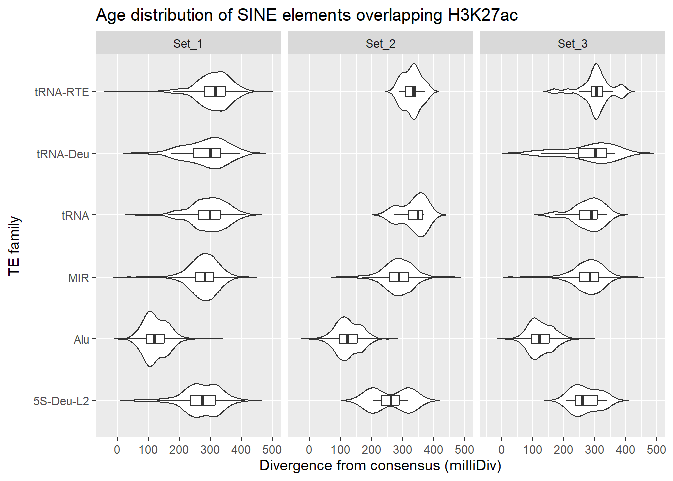

Past versions of "SINE Overlapping-1.png"

Version	Author	Date
68a0095	reneeisnowhere	2026-02-02

SINE_overlap_df %>% 
  dplyr::left_join(H3K27ac_lookup) %>% 
  dplyr::filter(cluster %in% c("Set_1","Set_2","Set_3")) %>% 
  ggplot(., aes(x = cluster, y = milliDiv)) +
  geom_violin(trim = FALSE) +
   geom_boxplot(width = 0.15, outlier.shape = NA) +
   coord_flip() +
   labs(
     y = "Divergence from consensus (milliDiv)",
     x = "TE family",
     title = "Age distribution of SINE elements overlapping H3K27ac"
   )+
  facet_wrap(~repName)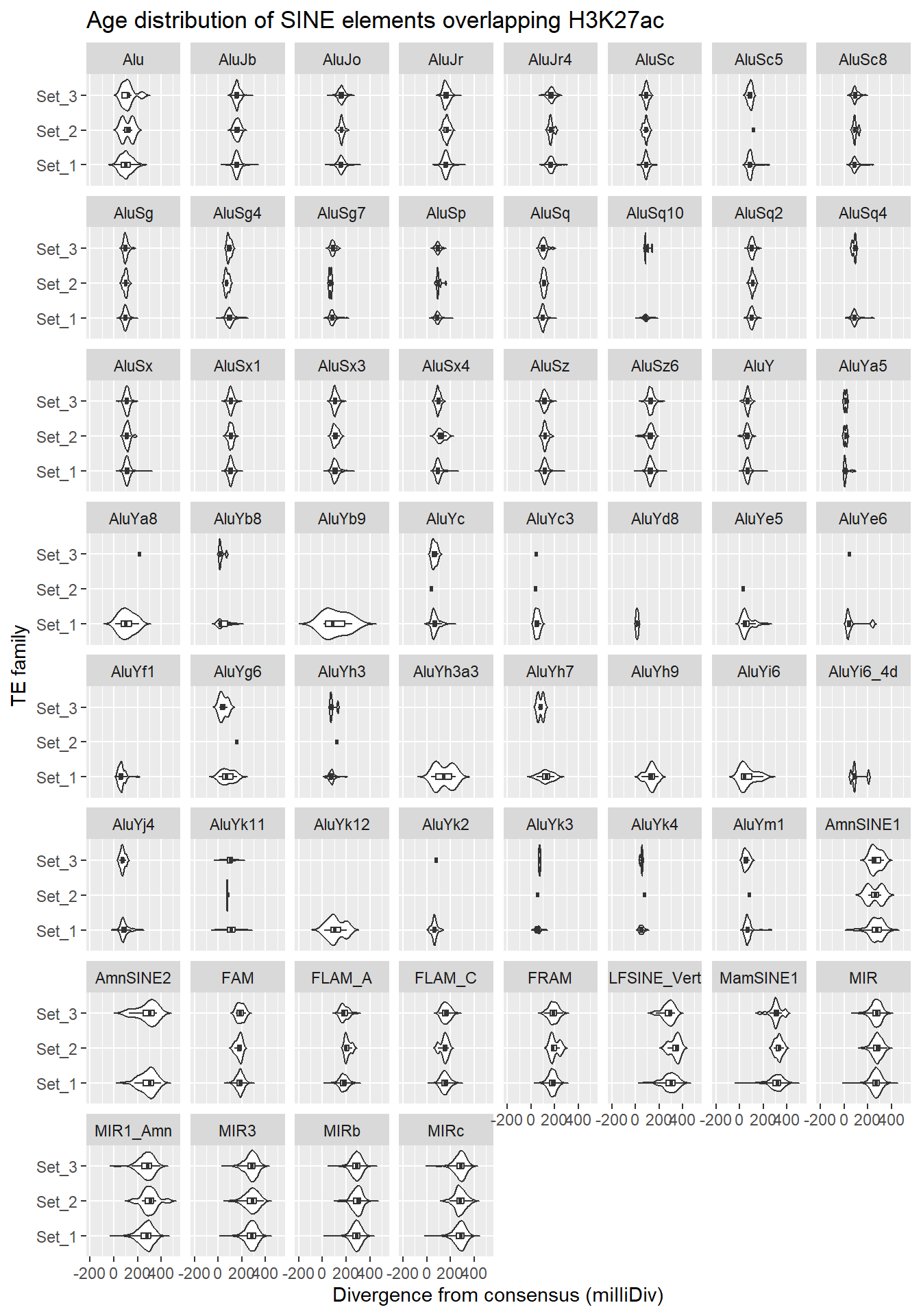

Past versions of "SINE Overlapping 2-1.png"

Version	Author	Date
68a0095	reneeisnowhere	2026-02-02

LINE

Overlapping LINE family with ROIs

LINE_hits <- findOverlaps(H3K27ac_sets_gr$all_H3K27ac, LINE_gr, ignore.strand = TRUE)

LINE_overlap_df <- tibble(
  peak_row = queryHits(LINE_hits),
  Peakid   = H3K27ac_sets_gr$all_H3K27ac$Peakid[queryHits(LINE_hits)],
  cluster  = H3K27ac_sets_gr$all_H3K27ac$cluster[queryHits(LINE_hits)],
  
  repClass = LINE_gr$repClass[subjectHits(LINE_hits)],
  repName  = LINE_gr$repName[subjectHits(LINE_hits)],
  
  TE_type  = ifelse(
    LINE_gr$repFamily[subjectHits(LINE_hits)] == "SVA",
    LINE_gr$repName[subjectHits(LINE_hits)],
    LINE_gr$repFamily[subjectHits(LINE_hits)]
  ),
  
  milliDiv = LINE_gr$milliDiv[subjectHits(LINE_hits)],
  milliDel = LINE_gr$milliDel[subjectHits(LINE_hits)],
  milliIns = LINE_gr$milliIns[subjectHits(LINE_hits)]
)

LINE_overlap_df %>% 
  dplyr::left_join(H3K27ac_lookup) %>% 
  dplyr::filter(cluster %in% c("Set_1","Set_2","Set_3")) %>% 
  ggplot(., aes(x = TE_type, y = milliDiv)) +
   geom_violin(trim = FALSE) +
   geom_boxplot(width = 0.15, outlier.shape = NA) +
   coord_flip() +
   labs(
     y = "Divergence from consensus (milliDiv)",
     x = "TE family",
     title = "Age distribution of LINE elements overlapping H3K27ac"
   )+
  facet_wrap(~cluster)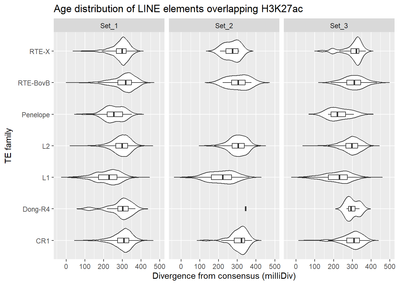

Past versions of "LINE Overlapping-1.png"

Version	Author	Date
68a0095	reneeisnowhere	2026-02-02

LTR

Overlapping LTR family with ROIs

LTR_hits <- findOverlaps(H3K27ac_sets_gr$all_H3K27ac, LTR_gr, ignore.strand = TRUE)

LTR_overlap_df <- tibble(
  peak_row = queryHits(LTR_hits),
  Peakid   = H3K27ac_sets_gr$all_H3K27ac$Peakid[queryHits(LTR_hits)],
  cluster  = H3K27ac_sets_gr$all_H3K27ac$cluster[queryHits(LTR_hits)],
  
  repClass = LTR_gr$repClass[subjectHits(LTR_hits)],
  repName  = LTR_gr$repName[subjectHits(LTR_hits)],
  RM_id  = LTR_gr$RM_id[subjectHits(LTR_hits)],
  TE_type  = ifelse(
    LTR_gr$repFamily[subjectHits(LTR_hits)] == "SVA",
    LTR_gr$repName[subjectHits(LTR_hits)],
    LTR_gr$repFamily[subjectHits(LTR_hits)]
  ),
  
  milliDiv = LTR_gr$milliDiv[subjectHits(LTR_hits)],
  milliDel = LTR_gr$milliDel[subjectHits(LTR_hits)],
  milliIns = LTR_gr$milliIns[subjectHits(LTR_hits)]
)

LTR_overlap_df %>% 
  dplyr::left_join(H3K27ac_lookup) %>% 
  dplyr::filter(cluster %in% c("Set_1","Set_2","Set_3")) %>% 
  ggplot(., aes(x = cluster, y = milliDiv)) +
   geom_violin(trim = FALSE) +
   geom_boxplot(width = 0.15, outlier.shape = NA) +
   coord_flip() +
   labs(
     y = "Divergence from consensus (milliDiv)",
     x = "TE family",
     title = "Age distribution of LTR elements overlapping H3K27ac"
   )+
  facet_wrap(~TE_type)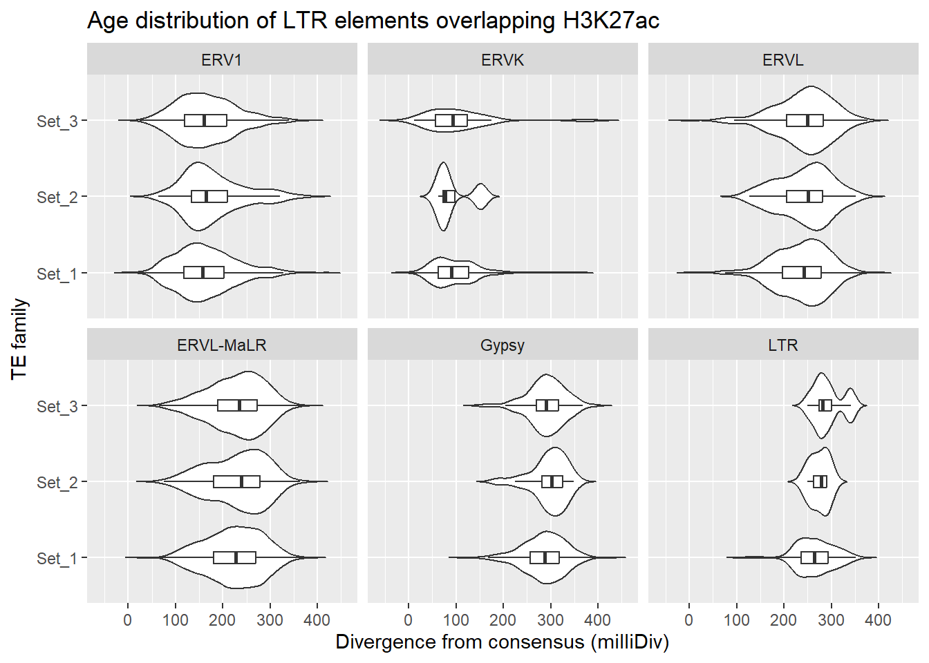

Past versions of "LTR Overlapping-1.png"

Version	Author	Date
81af285	reneeisnowhere	2026-02-04
68a0095	reneeisnowhere	2026-02-02

# saveRDS(LTR_overlap_df,"data/RDS_files/H3K27ac_Full_ROI_overlap_LTRs.RDS")

age tests

First test, within each TE family (ERVL, ERVK, etc…)do Set1,Set2 and Set3 differ?

age_kw <- LTR_overlap_df %>% 
  left_join(H3K27ac_lookup) %>% 
  filter(cluster %in% c("Set_1","Set_2","Set_3")) %>% 
  group_by(TE_type) %>% 
  summarise(
    kw_p = kruskal.test(milliDiv ~ cluster)$p.value)

age_kw

# A tibble: 6 × 2
  TE_type     kw_p
  <chr>      <dbl>
1 ERV1      0.0681
2 ERVK      0.945 
3 ERVL      0.0290
4 ERVL-MaLR 0.0223
5 Gypsy     0.211 
6 LTR       0.0482

The answer shows for ERVL, ERVL-MaLR, and LTR, yes age difference differ between sets. now to look at ERVL,ERVL-MaLR and LTR individually

test_TE_age_pairs <- function(df,
                              TE_type_query,
                              sets = c("Set_1", "Set_2", "Set_3")) {

  sub_df <- df %>% 
    dplyr::left_join(H3K27ac_lookup) %>% 
    dplyr::filter(
      TE_type == TE_type_query,
      cluster %in% sets,
      !is.na(milliDiv)
    )

  # Medians first (ground truth)
  med_df <- sub_df %>% 
    dplyr::group_by(cluster) %>% 
    dplyr::summarise(
      median_age = median(milliDiv, na.rm = TRUE),
      n = dplyr::n(),
      .groups = "drop"
    )

  # Pairwise Wilcoxon
  pw <- pairwise.wilcox.test(
    x = sub_df$milliDiv,
    g = sub_df$cluster,
    p.adjust.method = "BH"
  )

  # Tidy + enforce symmetric pairs
  pw_df <- as.data.frame(as.table(pw$p.value)) %>% 
    dplyr::filter(!is.na(Freq)) %>% 
    dplyr::rename(
      set_A = Var1,
      set_B = Var2,
      p_adj = Freq
    )

  # Join medians *by value*, not position
  pw_df %>% 
    dplyr::left_join(med_df, by = c("set_A" = "cluster")) %>% 
    dplyr::rename(median_A = median_age, n_A = n) %>% 
    dplyr::left_join(med_df, by = c("set_B" = "cluster")) %>% 
    dplyr::rename(median_B = median_age, n_B = n) %>% 
    dplyr::mutate(
      older_set = dplyr::case_when(
        median_A > median_B ~ set_A,
        median_B > median_A ~ set_B,
        TRUE ~ "equal"
      ),
      TE_type = TE_type_query
    )
}

test_TE_age_pairs(LTR_overlap_df, "ERV1")

  set_A set_B      p_adj median_A n_A median_B  n_B older_set TE_type
1 Set_2 Set_1 0.09778575      165 107      157 6385     Set_2    ERV1
2 Set_3 Set_1 0.33055165      160 642      157 6385     Set_3    ERV1
3 Set_3 Set_2 0.14838385      160 642      165  107     Set_2    ERV1

test_TE_age_pairs(LTR_overlap_df, "ERVK")

  set_A set_B p_adj median_A n_A median_B n_B older_set TE_type
1 Set_2 Set_1     1       77   4       90 537     Set_1    ERVK
2 Set_3 Set_1     1       93  25       90 537     Set_3    ERVK
3 Set_3 Set_2     1       93  25       77   4     Set_3    ERVK

test_TE_age_pairs(LTR_overlap_df, "ERVL")

  set_A set_B      p_adj median_A n_A median_B  n_B older_set TE_type
1 Set_2 Set_1 0.42714314      251  91      242 6318     Set_2    ERVL
2 Set_3 Set_1 0.04056578      250 504      242 6318     Set_3    ERVL
3 Set_3 Set_2 0.99418468      250 504      251   91     Set_2    ERVL

test_TE_age_pairs(LTR_overlap_df, "ERVL-MaLR")

  set_A set_B      p_adj median_A n_A median_B   n_B older_set   TE_type
1 Set_2 Set_1 0.17332708      239 197      227 10698     Set_2 ERVL-MaLR
2 Set_3 Set_1 0.06074938      235 945      227 10698     Set_3 ERVL-MaLR
3 Set_3 Set_2 0.60549175      235 945      239   197     Set_2 ERVL-MaLR

test_TE_age_pairs(LTR_overlap_df, "LTR")

  set_A set_B      p_adj median_A n_A median_B n_B older_set TE_type
1 Set_2 Set_1 0.56351607    278.5   4    264.0  92     Set_2     LTR
2 Set_3 Set_1 0.04873491    282.0  13    264.0  92     Set_3     LTR
3 Set_3 Set_2 0.46137897    282.0  13    278.5   4     Set_3     LTR

DNA

Overlapping DNA family with ROIs

DNA_hits <- findOverlaps(H3K27ac_sets_gr$all_H3K27ac, DNA_gr, ignore.strand = TRUE)

DNA_overlap_df <- tibble(
  peak_row = queryHits(DNA_hits),
  Peakid   = H3K27ac_sets_gr$all_H3K27ac$Peakid[queryHits(DNA_hits)],
  cluster  = H3K27ac_sets_gr$all_H3K27ac$cluster[queryHits(DNA_hits)],
  
  repClass = DNA_gr$repClass[subjectHits(DNA_hits)],
  repName  = DNA_gr$repName[subjectHits(DNA_hits)],
  
  TE_type  = ifelse(
    DNA_gr$repFamily[subjectHits(DNA_hits)] == "SVA",
    DNA_gr$repName[subjectHits(DNA_hits)],
    DNA_gr$repFamily[subjectHits(DNA_hits)]
  ),
  
  milliDiv = DNA_gr$milliDiv[subjectHits(DNA_hits)],
  milliDel = DNA_gr$milliDel[subjectHits(DNA_hits)],
  milliIns = DNA_gr$milliIns[subjectHits(DNA_hits)]
)

DNA_overlap_df %>% 
  dplyr::left_join(H3K27ac_lookup) %>% 
  dplyr::filter(cluster %in% c("Set_1","Set_2","Set_3")) %>% 
  ggplot(., aes(x = TE_type, y = milliDiv)) +
   geom_violin(trim = FALSE) +
   geom_boxplot(width = 0.15, outlier.shape = NA) +
   coord_flip() +
   labs(
     y = "Divergence from consensus (milliDiv)",
     x = "TE family",
     title = "Age distribution of DNA elements overlapping H3K27ac"
   )+
  facet_wrap(~cluster)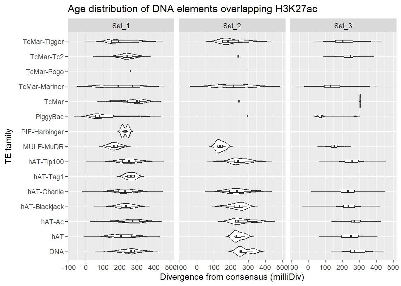

Past versions of "DNA Overlapping-1.png"

Version	Author	Date
68a0095	reneeisnowhere	2026-02-02

SVA/Retroposon

Overlapping SVA family with ROIs

SVA_hits <- findOverlaps(H3K27ac_sets_gr$all_H3K27ac, SVA_gr, ignore.strand = TRUE)

SVA_overlap_df <- tibble(
  peak_row = queryHits(SVA_hits),
  Peakid   = H3K27ac_sets_gr$all_H3K27ac$Peakid[queryHits(SVA_hits)],
  cluster  = H3K27ac_sets_gr$all_H3K27ac$cluster[queryHits(SVA_hits)],
  
  repClass = SVA_gr$repClass[subjectHits(SVA_hits)],
  repName  = SVA_gr$repName[subjectHits(SVA_hits)],
  
  TE_type  = ifelse(
    SVA_gr$repFamily[subjectHits(SVA_hits)] == "SVA",
    SVA_gr$repName[subjectHits(SVA_hits)],
    SVA_gr$repFamily[subjectHits(SVA_hits)]
  ),
  
  milliDiv = SVA_gr$milliDiv[subjectHits(SVA_hits)],
  milliDel = SVA_gr$milliDel[subjectHits(SVA_hits)],
  milliIns = SVA_gr$milliIns[subjectHits(SVA_hits)]
)

SVA_overlap_df %>% 
  dplyr::left_join(H3K27ac_lookup) %>% 
  dplyr::filter(cluster %in% c("Set_1","Set_2","Set_3")) %>% 
  ggplot(., aes(x = TE_type, y = milliDiv)) +
   geom_violin(trim = FALSE) +
   geom_boxplot(width = 0.15, outlier.shape = NA) +
   coord_flip() +
   labs(
     y = "Divergence from consensus (milliDiv)",
     x = "TE family",
     title = "Age distribution of SVA elements overlapping H3K27ac"
   )+
  facet_wrap(~cluster)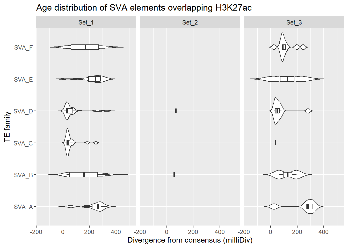

Past versions of "SVA Overlapping-1.png"

Version	Author	Date
68a0095	reneeisnowhere	2026-02-02

Looking for overlapping information: LTR specific

Here I am exploring H3K27ac ROIs which overlap LTRs and also overlap H3K9me3 ROIs, then exploring LFC of the H3K27ac ROI sets across families of LTRs. First I wanted to know how many H3K27ac ROIs overlap LTRs, and how many of those LTRs overlap more than one ROI:

LTR_overlap_df %>% 
  count(Peakid, name = "n_peaks") %>%
  count(n_peaks)

# A tibble: 12 × 2
   n_peaks     n
     <int> <int>
 1       1 18389
 2       2  4997
 3       3  1468
 4       4   432
 5       5   144
 6       6    56
 7       7    26
 8       8     8
 9       9     8
10      10     3
11      11     1
12      12     1

LTR_only_K27ac_peakids <- LTR_overlap_df %>% distinct(Peakid)

I then overlapped ROIs with H3K9me3 ROIs to see how many H3K9me3 ROIs overlap H3K27ac ROIs. (interpret with n_peaks being how many H3K27ac ROIs and n being number of H3K9me3 ROIS, So 33,567 K9me3 rOIs overlap 1 H3K27me3

K9me3_hits <- findOverlaps(H3K27ac_sets_gr$all_H3K27ac, H3K9me3_sets_gr$all_H3K9me3_regions, ignore.strand = TRUE)

K9me3_overlap_df <- tibble(
  peak_row = queryHits(K9me3_hits),
  Peakid   = H3K27ac_sets_gr$all_H3K27ac$Peakid[queryHits(K9me3_hits)],
  cluster  = H3K27ac_sets_gr$all_H3K27ac$cluster[queryHits(K9me3_hits)],
  ROI_K9me3 = H3K9me3_sets_gr$all_H3K9me3_regions$Peakid[subjectHits(K9me3_hits)])

K9me3_overlap_df %>%
  count(Peakid, name = "n_peaks") %>%
  count(n_peaks)

# A tibble: 17 × 2
   n_peaks     n
     <int> <int>
 1       1 33567
 2       2  5184
 3       3  1072
 4       4   303
 5       5   161
 6       6    59
 7       7    38
 8       8    20
 9       9    11
10      10     8
11      11    12
12      12     3
13      13     4
14      14     1
15      15     4
16      16     3
17      17     2

K9me3_only_K27ac_peakids <- K9me3_overlap_df %>% distinct(Peakid)

Now to filter and connect H3K27ac ROIs, that overlap LTRs and at least one H3K9me3

LTR_overlap_df %>% 
  dplyr::filter(Peakid %in% K9me3_only_K27ac_peakids$Peakid) %>%  distinct(RM_id)

# A tibble: 12,645 × 1
   RM_id                 
   <chr>                 
 1 chr1:1003379-1003425:1
 2 chr1:1003500-1003623:1
 3 chr1:1005447-1005607:1
 4 chr1:1017170-1018876:1
 5 chr1:1214911-1215005:1
 6 chr1:1235837-1235999:1
 7 chr1:1259547-1259908:1
 8 chr1:1357233-1357526:1
 9 chr1:1357817-1357890:1
10 chr1:1382090-1382288:1
# ℹ 12,635 more rows

LFC of those regions

LTR_overlap_df %>% 
  dplyr::filter(Peakid %in% K9me3_only_K27ac_peakids$Peakid) %>% 
  
  left_join(., K27ac_lfctable, by = c("Peakid"="genes")) %>% 
  group_by(TE_type) %>% 
  tally() %>% 
   ungroup() %>% 
  DT::datatable(
    rownames = FALSE,
    caption = htmltools::tags$caption(
      style = "caption-side: top; text-align: left;",
      "H3K27ac LTR specific overlap counts by TE familiy which also overlap H3K9me3"),
    options = list(pageLength = 10,
      autoWidth = TRUE,
      dom = "tip"))

LTR_overlap_df %>% 
  dplyr::left_join(H3K27ac_lookup) %>% 
   dplyr::filter(Peakid %in% K9me3_only_K27ac_peakids$Peakid) %>% 
  dplyr::filter(cluster %in% c("Set_1","Set_2","Set_3")) %>% 
  ggplot(., aes(x = TE_type, y = milliDiv)) +
   geom_violin(trim = FALSE) +
   geom_boxplot(width = 0.15, outlier.shape = NA) +
   coord_flip() +
   labs(
     y = "Divergence from consensus (milliDiv)",
     x = "TE family",
     title = "Age distribution of LTR elements overlapping H3K27ac and H3K9me3"
   )+
  facet_wrap(~cluster)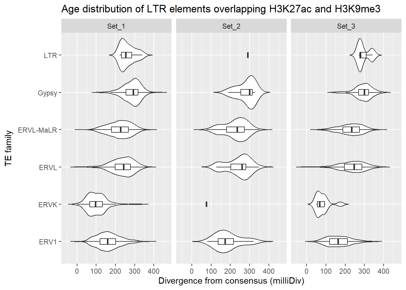

Past versions of unnamed-chunk-8-1.png

Version	Author	Date
81af285	reneeisnowhere	2026-02-04

LTR_K9me3_H3K27ac_lfc <- LTR_overlap_df %>% 
   left_join(., K27ac_lfctable, by = c("Peakid"="genes")) %>%
   dplyr::filter(Peakid %in% K9me3_only_K27ac_peakids$Peakid)

plot_K27_family <- function(lfc_df,
                            grp="H3K27ac",
                            repFamily,
                            fam_name){

  lfc_df %>% 
  dplyr::filter(Peakid %in% K9me3_only_K27ac_peakids$Peakid) %>% 
    dplyr::filter(.data$TE_type %in% fam_name) %>% 
  dplyr::filter(cluster != "NA") %>% 
  pivot_longer(.,cols=c(starts_with(grp)), names_to="group", values_to = "LFC") %>% 
  group_by(cluster, group) %>%
  summarise(median_abs_LFC = median(abs(LFC), na.rm = TRUE),
            .groups = "drop")%>% 
  mutate(time=str_remove(group,grp))%>% 
  mutate(time=factor(time, levels=c("_24T","_24R","_144R"))) %>% 
  ggplot(., aes(x=time, y=median_abs_LFC, group=cluster, color=cluster))+
  geom_point(size=4)+
  geom_line(aes(alpha = 0.8, linewidth = 4))+
  theme_bw()+
  ggtitle(paste0(grp," absolute LFC overlapping ",repFamily,":",fam_name))
}

plot_K27_family(LTR_K9me3_H3K27ac_lfc,"H3K27ac","LTR","ERV1")+
  scale_color_manual(values = cluster_colors, drop = FALSE)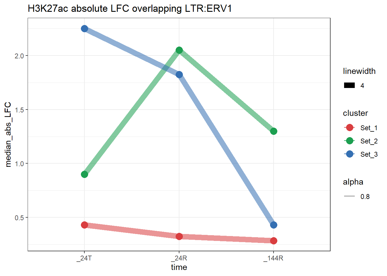

Past versions of "LTR lfc H3K9me3-1.png"

Version	Author	Date
68a0095	reneeisnowhere	2026-02-02

plot_K27_family(LTR_K9me3_H3K27ac_lfc,"H3K27ac","LTR","ERVK")+
  scale_color_manual(values = cluster_colors, drop = FALSE)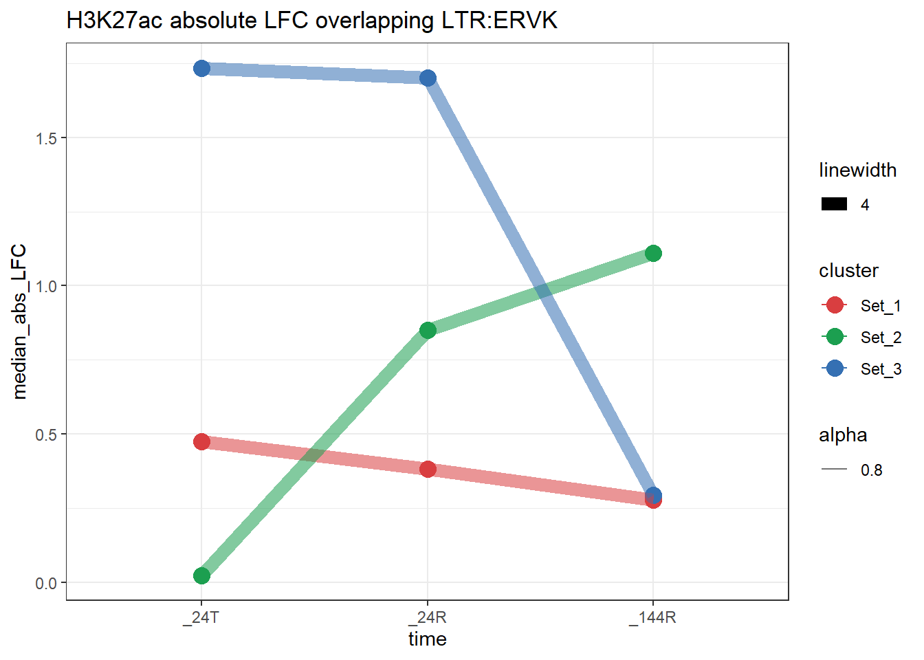

Past versions of "LTR lfc H3K9me3-2.png"

Version	Author	Date
68a0095	reneeisnowhere	2026-02-02

plot_K27_family(LTR_K9me3_H3K27ac_lfc,"H3K27ac","LTR","ERVL")+
  scale_color_manual(values = cluster_colors, drop = FALSE)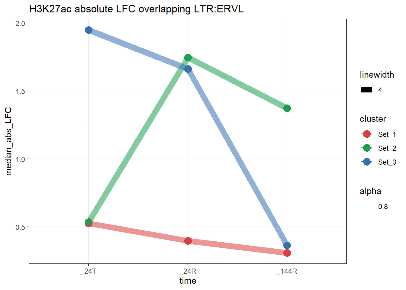

Past versions of "LTR lfc H3K9me3-3.png"

Version	Author	Date
68a0095	reneeisnowhere	2026-02-02

plot_K27_family(LTR_K9me3_H3K27ac_lfc,"H3K27ac","LTR","Gypsy")+
  scale_color_manual(values = cluster_colors, drop = FALSE)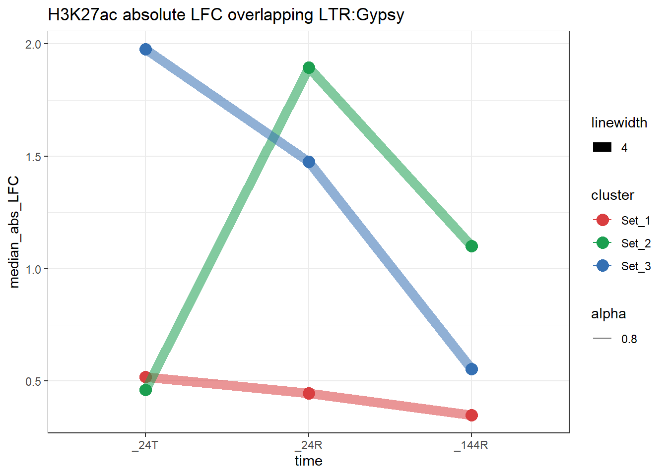

Past versions of "LTR lfc H3K9me3-4.png"

Version	Author	Date
68a0095	reneeisnowhere	2026-02-02

plot_K27_family(LTR_K9me3_H3K27ac_lfc,"H3K27ac","LTR","ERVL-MaLR")+
  scale_color_manual(values = cluster_colors, drop = FALSE)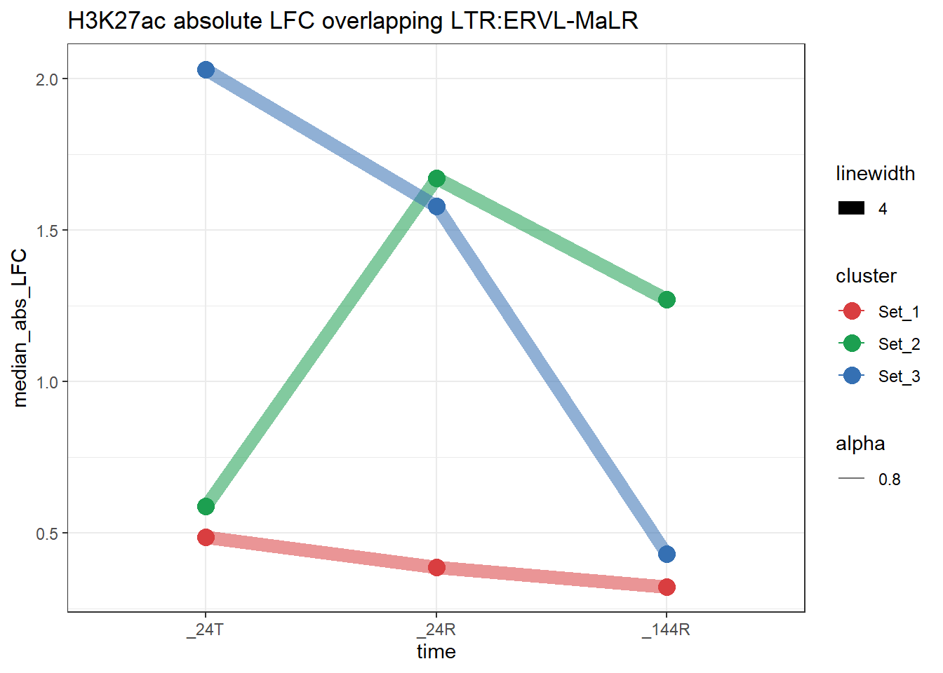

Past versions of "LTR lfc H3K9me3-5.png"

Version	Author	Date
68a0095	reneeisnowhere	2026-02-02

plot_K27_family(LTR_K9me3_H3K27ac_lfc,"H3K27ac","LTR","LTR")+
  scale_color_manual(values = cluster_colors, drop = FALSE)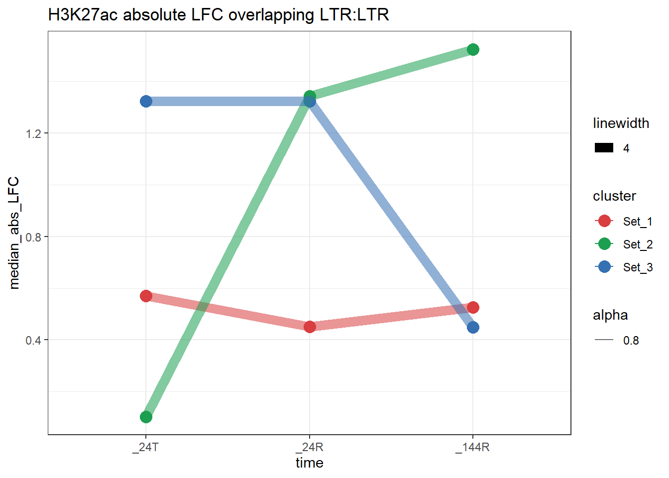

Past versions of "LTR lfc H3K9me3-6.png"

Version	Author	Date
68a0095	reneeisnowhere	2026-02-02

Raw LFC exploration

This will look at Raw LFC for all H3K27ac ROIs that overlap an LTR

LTR_overlap_df %>% 
  
   left_join(., K27ac_lfctable, by = c("Peakid"="genes")) %>% 
  pivot_longer(.,cols=c(starts_with("H3K27ac")), names_to="group", values_to = "LFC") %>% 
  group_by(cluster, group) %>%
  # summarise(median_LFC = median(LFC), na.rm = TRUE),
  #           .groups = "drop")%>% 
  dplyr::filter(cluster=="Set_2") %>% 
   mutate(time=str_remove(group,"H3K27ac"))%>% 
  mutate(time=factor(time, levels=c("_24T","_24R","_144R")))  %>% 
  ggplot(., aes(x=time, y = LFC, group=Peakid))+
  geom_line(alpha = 0.3) +
  geom_point(size = 1) +
  theme_classic() +
  labs(
    x = "Time point",
    y = "Log2 Fold Change",
    title = "H3K27ac LFC  for Set_2 LTR-overlapping regions")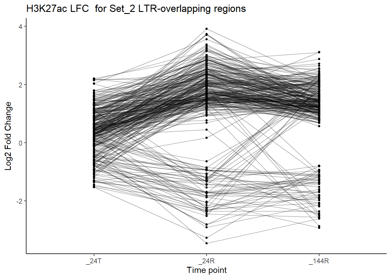

Past versions of unnamed-chunk-10-1.png

Version	Author	Date
81af285	reneeisnowhere	2026-02-04

LTR_overlap_df %>% 
   left_join(., K27ac_lfctable, by = c("Peakid"="genes")) %>% 
  pivot_longer(.,cols=c(starts_with("H3K27ac")), names_to="group", values_to = "LFC") %>% 
  group_by(cluster, group) %>%
  # summarise(median_LFC = median(LFC), na.rm = TRUE),
  #           .groups = "drop")%>% 
  # dplyr::filter(cluster=="Set_3") %>% 
   mutate(time=str_remove(group,"H3K27ac"))%>% 
  mutate(time=factor(time, levels=c("_24T","_24R","_144R")))  %>% 
  ggplot(., aes(x=time, y = LFC, group=Peakid, color=case))+
  geom_line(alpha = 0.3) +
  geom_point(size = 1) +
  theme_classic() +
  facet_wrap(~cluster)+
  labs(
    x = "Time point",
    y = "Log2 Fold Change",
    title = "H3K27ac LFC  for all LTR-overlapping regions")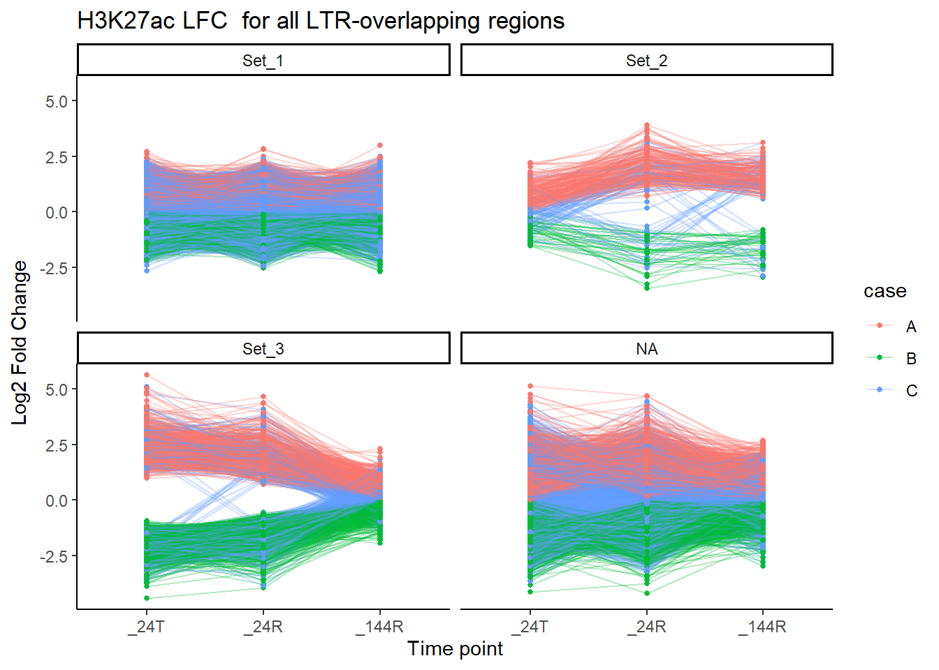

Past versions of unnamed-chunk-10-2.png

Version	Author	Date
81af285	reneeisnowhere	2026-02-04

Getting some number about how many, etc…

LTR_overlap_df %>% 
  dplyr::left_join(H3K27ac_lookup) %>% 
  group_by(TE_type,cluster) %>% 
  tally() %>% 
  pivot_wider(id_cols = TE_type, names_from = cluster, values_from = n) %>% 
  ungroup() %>% 
  DT::datatable(
    rownames = FALSE,
    caption = htmltools::tags$caption(
      style = "caption-side: top; text-align: left;",
      "H3K27ac LTR specific overlap counts by TE familiy"),
    options = list(pageLength = 10,
      autoWidth = TRUE,
      dom = "tip"))

now breaking out by family

LTR_overlap_df %>% 
   left_join(., K27ac_lfctable, by = c("Peakid"="genes")) %>% 
  pivot_longer(.,cols=c(starts_with("H3K27ac")), names_to="group", values_to = "LFC") %>% 
  group_by(cluster, group) %>%
  # summarise(median_LFC = median(LFC), na.rm = TRUE),
  #           .groups = "drop")%>% 
  dplyr::filter(cluster=="Set_2") %>% 
   mutate(time=str_remove(group,"H3K27ac"))%>% 
  mutate(time=factor(time, levels=c("_24T","_24R","_144R")))  %>% 
  ggplot(., aes(x=time, y = LFC, group=Peakid, color=case))+
  geom_line(alpha = 0.3) +
  geom_point(size = 1) +
  theme_classic() +
  facet_wrap(~TE_type)+
  labs(
    x = "Time point",
    y = "Log2 Fold Change",
    title = "H3K27ac LFC  for Set_2 LTR-overlapping regions")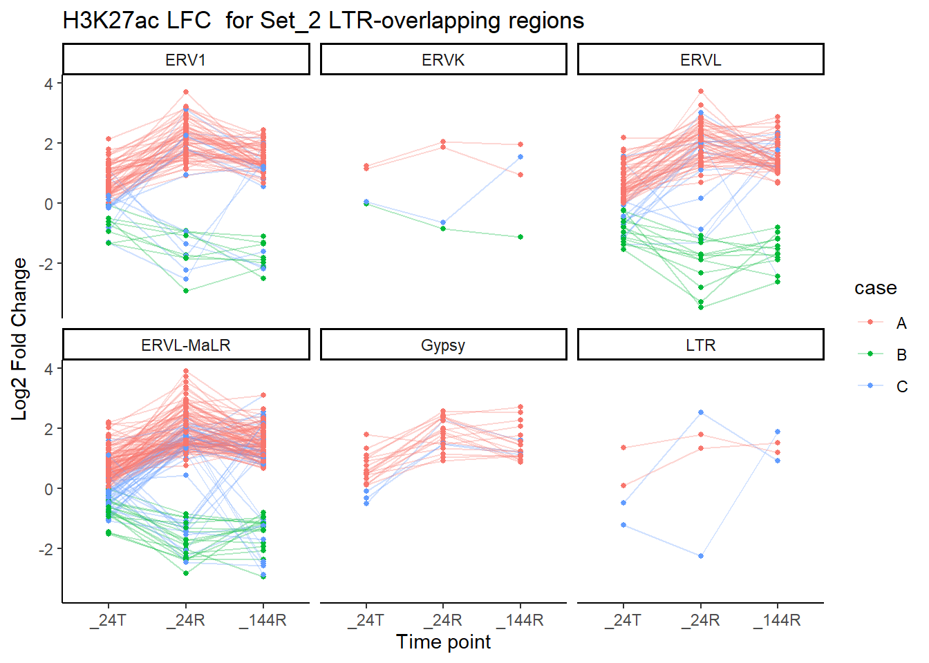

Past versions of unnamed-chunk-12-1.png

Version	Author	Date
81af285	reneeisnowhere	2026-02-04

LTR_overlap_df %>% 
  left_join(., K27ac_lfctable, by = c("Peakid"="genes")) %>% 
  pivot_longer(.,cols=c(starts_with("H3K27ac")), names_to="group", values_to = "LFC") %>% 
  group_by(cluster, group) %>%
  # summarise(median_LFC = median(LFC), na.rm = TRUE),
  #           .groups = "drop")%>% 
  dplyr::filter(cluster=="Set_3") %>% 
   mutate(time=str_remove(group,"H3K27ac"))%>% 
  mutate(time=factor(time, levels=c("_24T","_24R","_144R")))  %>% 
  ggplot(., aes(x=time, y = LFC, group=Peakid, color=case))+
  geom_line(alpha = 0.3) +
  geom_point(size = 1) +
  theme_classic() +
  facet_wrap(~TE_type)+
  labs(
    x = "Time point",
    y = "Log2 Fold Change",
    title = "H3K27ac LFC  for Set_3 LTR-overlapping regions")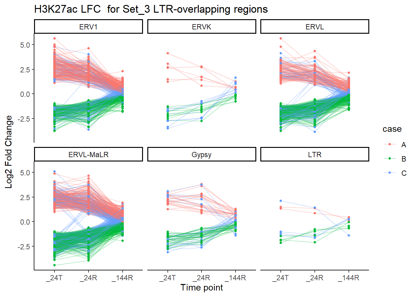

Past versions of unnamed-chunk-12-2.png

Version	Author	Date
81af285	reneeisnowhere	2026-02-04

There appears to be a lot of variation on LFC. Direction is obscuring information. I am now attempting to create a list of ROIs by set where LFC across time is always >0 (The up group), another set where LFC across time is always <0 (The down group), and the catch all mixed group.

### already added to the K27ac_lfctable
# LTR_overlap_df %>% 
#   dplyr::left_join(H3K27ac_lookup) %>% 
#    left_join(., K27ac_lfctable, by = c("Peakid"="genes")) %>% 
#    mutate(case= case_when(H3K27ac_24T > 0 & H3K27ac_24R >0 & H3K27ac_144R>0~"A",
#                               H3K27ac_24T < 0 & H3K27ac_24R <0 & H3K27ac_144R<0~"B",
#                               TRUE ~ "C")) %>% 
#   mutate(set_case=paste0(cluster,"_",case))
median_df <- K27ac_lfctable %>% 
  pivot_longer(.,cols=c(starts_with("H3K27ac")), names_to="group", values_to = "LFC") %>% 
  mutate(
    time = stringr::str_remove(group, "H3K27ac"),
    time = factor(time, levels = c("_24T", "_24R", "_144R"))
  ) %>%
  group_by(cluster, time) %>% 
  summarise(
    median_LFC = median(LFC, na.rm = TRUE),
    n_peaks = dplyr::n(),
    .groups = "drop")
  
K27ac_lfctable %>% 
  pivot_longer(.,cols=c(starts_with("H3K27ac")), names_to="group", values_to = "LFC") %>% 
   mutate(time=str_remove(group,"H3K27ac"))%>% 
  mutate(time=factor(time, levels=c("_24T","_24R","_144R")))  %>% 
  ggplot(., aes(x=time, y = LFC, group=genes, color=case))+
  ggrastr::rasterise(geom_line(alpha = 0.15)) +
  ggrastr::geom_point_rast(size = 1) +
  geom_line(data=median_df, aes(x=time, y=median_LFC, group = cluster),inherit.aes = FALSE, linewidth =2)+
  theme_classic() +
  facet_wrap(~cluster)+
  labs(
    x = "Time point",
    y = "Log2 Fold Change",
    title = "H3K27ac LFC  for all H3K27ac regions")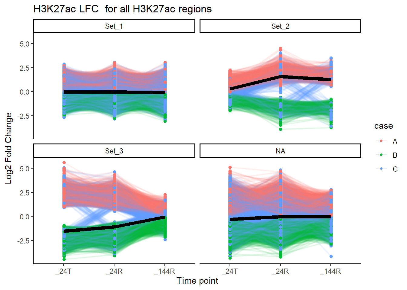

Past versions of "split groups by LFC-1.png"

Version	Author	Date
3fa291d	reneeisnowhere	2026-02-03

K27ac_lfctable %>% 
  pivot_longer(.,cols=c(starts_with("H3K27ac")), names_to="group", values_to = "LFC") %>% 
   mutate(time=str_remove(group,"H3K27ac"))%>% 
  mutate(time=factor(time, levels=c("_24T","_24R","_144R")))  %>% 
  ggplot(., aes(x=time, y = LFC, group=genes))+
  ggrastr::rasterise(geom_line(alpha = 0.15,color="darkgray")) +
  ggrastr::geom_point_rast(size = 1) +
  geom_line(data=median_df, aes(x=time, y=median_LFC, group = cluster),inherit.aes = FALSE, linewidth =2)+
  theme_classic() +
  facet_wrap(~cluster)+
  labs(
    x = "Time point",
    y = "Log2 Fold Change",
    title = "H3K27ac LFC  for all H3K27ac regions")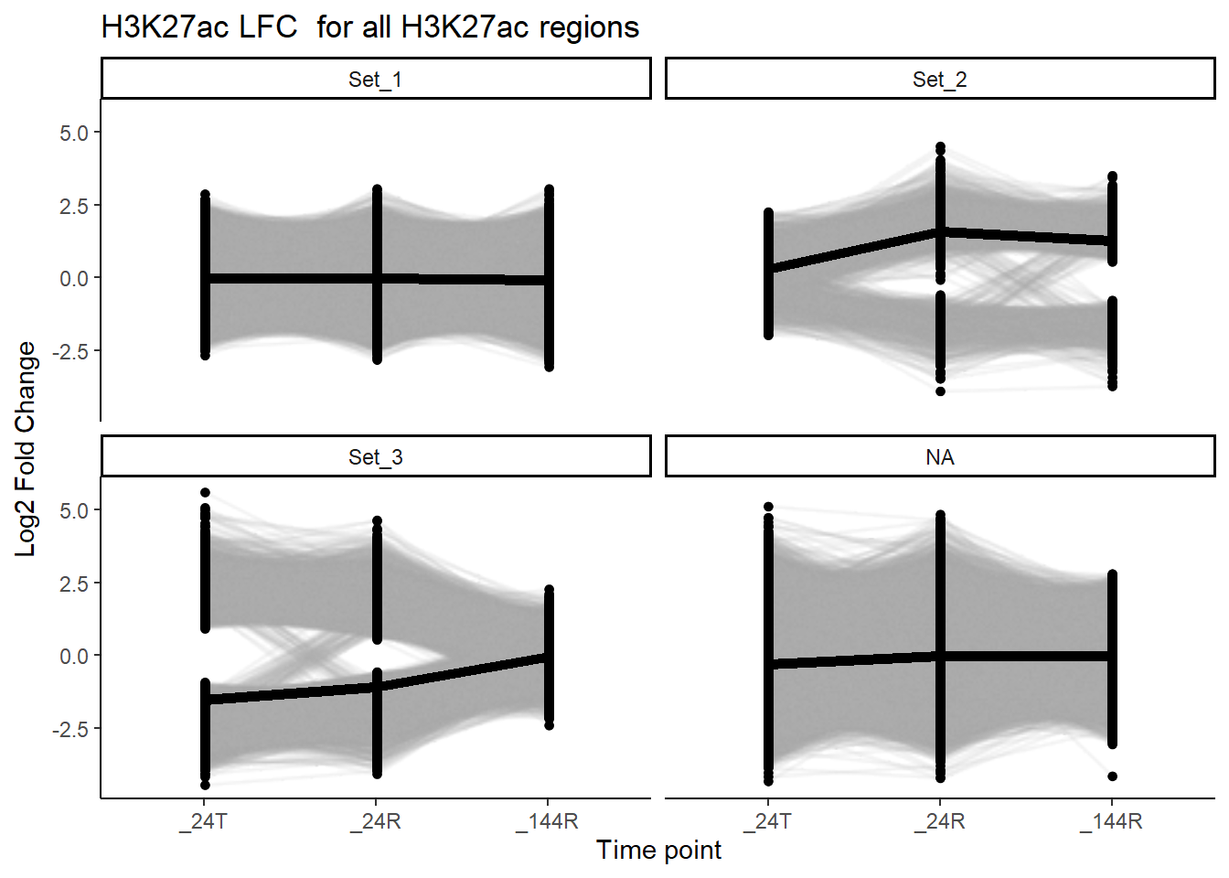

Past versions of "split groups by LFC-2.png"

Version	Author	Date
9a1e513	reneeisnowhere	2026-02-17
1a85f13	reneeisnowhere	2026-02-17

K27ac_lfctable %>% 
  group_by(cluster,case) %>% 
  tally() %>% pivot_wider(id_cols=case, names_from = cluster, values_from = n) %>% 
  mutate(type=case_when(case=="A"~"All LFC > 0",
                        case=="B" ~ "All LFC < 0",
                        case=="C"~"Mixed up and down LFC")) %>% 
  DT::datatable(
    rownames = FALSE,
    caption = htmltools::tags$caption(
      style = "caption-side: top; text-align: left;",
      "H3K27ac ROI counts stratified by LFC case"),
    options = list(pageLength = 10,
      autoWidth = TRUE,
      dom = "tip"))

H3K27ac_Sets <- K27ac_lfctable %>%
  dplyr::rename("Peakid"=genes)

H3K27ac_set_case_lfc <- split(H3K27ac_Sets, H3K27ac_Sets$set_case)

# saveRDS(H3K27ac_set_case_lfc, "data/RDS_files/H3K27ac_set_case_lfc.RDS")
unique(rpt_split$`LTR`$repFamily)

Zooming back in on summits,

What do LFCs of ROIs whose summits cross LTRs?

toss <- findOverlaps(H3K27ac_summit_gr, LTR_gr)
# toss %>% 
#   as.data.frame() %>% 
#   distinct(Peakid)
LTR_summits_overlap_df <- tibble(
  peak_row = queryHits(toss),
  Peakid   = H3K27ac_summit_gr$Peakid[queryHits(toss)],
  cluster  = H3K27ac_sets_gr$cluster[queryHits(toss)],
  
  repClass = LTR_gr$repClass[subjectHits(toss)],
  repName  = LTR_gr$repName[subjectHits(toss)],
  RM_id  = LTR_gr$RM_id[subjectHits(toss)],
  TE_type  = ifelse(
    LTR_gr$repFamily[subjectHits(toss)] == "SVA",
    LTR_gr$repName[subjectHits(toss)],
    LTR_gr$repFamily[subjectHits(toss)]
  ),
  
  milliDiv = LTR_gr$milliDiv[subjectHits(toss)],
  milliDel = LTR_gr$milliDel[subjectHits(toss)],
  milliIns = LTR_gr$milliIns[subjectHits(toss)]
)
summit_LTR_peakids <- LTR_summits_overlap_df %>% distinct(Peakid)

split_summit_LTR_peakids <- split(LTR_summits_overlap_df, LTR_summits_overlap_df$TE_type)

saveRDS(LTR_summits_overlap_df,"data/RDS_files/H3K27ac_summit_LTR_overlaps.RDS")

med_LTR_LFC <- K27ac_lfctable %>% 
  dplyr::filter(genes %in% summit_LTR_peakids$Peakid) %>% 
  pivot_longer(.,cols=c(starts_with("H3K27ac")), names_to="group", values_to = "LFC") %>% 
   mutate(
    time = stringr::str_remove(group, "H3K27ac"),
    time = factor(time, levels = c("_24T", "_24R", "_144R"))
  ) %>%
  group_by(cluster, time) %>% 
  summarise(
    median_LFC = median(LFC, na.rm = TRUE),
    n_peaks = dplyr::n(),
    .groups = "drop")


K27ac_lfctable %>% 
  dplyr::filter(genes %in% summit_LTR_peakids$Peakid) %>% 
  pivot_longer(.,cols=c(starts_with("H3K27ac")), names_to="group", values_to = "LFC") %>% 
   mutate(time=str_remove(group,"H3K27ac"))%>% 
  mutate(time=factor(time, levels=c("_24T","_24R","_144R")))  %>% 
  ggplot(., aes(x=time, y = LFC, group=genes, color=case))+
  ggrastr::rasterise(geom_line(alpha = 0.15)) +
  ggrastr::geom_point_rast(size = 1) +
  geom_line(data=med_LTR_LFC, aes(x=time, y=median_LFC, group = cluster),inherit.aes = FALSE, linewidth =2)+
  theme_classic() +
  facet_wrap(~cluster)+
  labs(
    x = "Time point",
    y = "Log2 Fold Change",
    title = "H3K27ac LFC for all H3K27ac regions whose summits cross an LTR")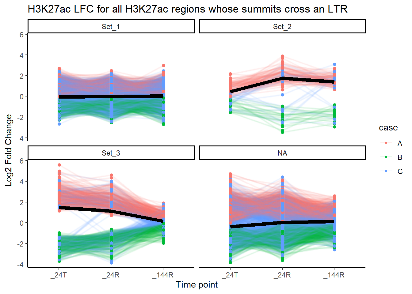

Past versions of "All LTRs and summits-1.png"

Version	Author	Date
81af285	reneeisnowhere	2026-02-04

median_LFC_H3K27ac_group_plot <- function(lfc_df,repFam){

  pid_df <- split_summit_LTR_peakids[[repFam]]

  med_df <- lfc_df %>% 
  dplyr::filter(genes %in% pid_df$Peakid) %>%
  pivot_longer(.,cols=c(starts_with("H3K27ac")), names_to="group", values_to = "LFC") %>% 
  mutate(
    time = stringr::str_remove(group, "H3K27ac"),
    time = factor(time, levels = c("_24T", "_24R", "_144R"))
  ) %>%
  group_by(cluster, time) %>% 
  summarise(
    median_LFC = median(LFC, na.rm = TRUE),
    n_peaks = dplyr::n(),
    .groups = "drop")
  
  label_df <- med_df %>%
  group_by(cluster) %>%
  summarise(n_peaks = unique(n_peaks),   # same for all times within a cluster
    .groups = "drop") %>%
  mutate(label = paste0("n = ", n_peaks),
    time = "_144R",               # anchor text at first x position
    y = Inf )  ##place at top of panel


  lfc_df %>% 
  dplyr::filter(genes %in% pid_df$Peakid) %>%
  pivot_longer(.,cols=c(starts_with("H3K27ac")), names_to="group", values_to = "LFC") %>% 
   mutate(time=str_remove(group,"H3K27ac"))%>% 
  mutate(time=factor(time, levels=c("_24T","_24R","_144R")))  %>% 
  ggplot(., aes(x=time, y = LFC, group=genes, color=case))+
  ggrastr::rasterise(geom_line(alpha = 0.15)) +
  ggrastr::geom_point_rast(size = 1) +
  geom_line(data=med_df, aes(x=time, y=median_LFC, group = cluster),inherit.aes = FALSE, linewidth =2)+
    geom_text(data = label_df,  aes(x = time, y = y, label = label),  inherit.aes = FALSE,  vjust = 1.2,  hjust = .2,  size = 4)+
  theme_classic() +
  facet_wrap(~cluster)+
  labs(
    x = "Time point",
    y = "Log2 Fold Change",
    title = paste0("H3K27ac LFC, ROI summits cross an LTR:",repFam))
  }

median_LFC_H3K27ac_group_plot(K27ac_lfctable,"ERVL-MaLR")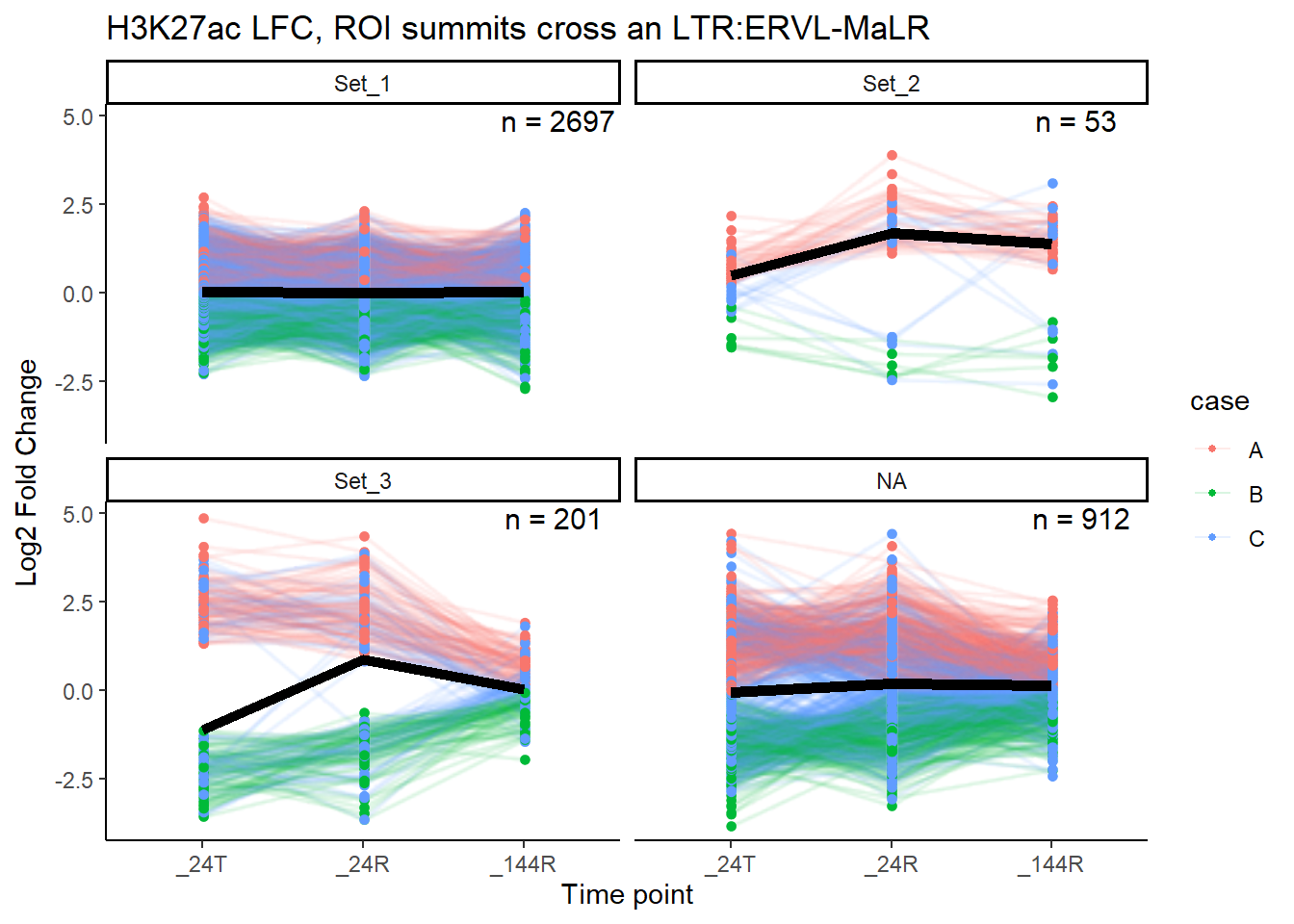

Past versions of "All LTRs and summits ERV1-1.png"

Version	Author	Date
81af285	reneeisnowhere	2026-02-04

median_LFC_H3K27ac_group_plot(K27ac_lfctable,"ERV1")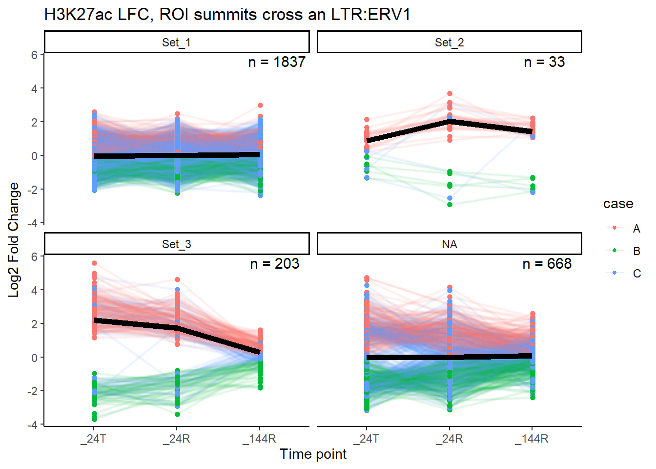

Past versions of "All LTRs and summits ERV1-2.png"

Version	Author	Date
81af285	reneeisnowhere	2026-02-04

median_LFC_H3K27ac_group_plot(K27ac_lfctable,"ERVL")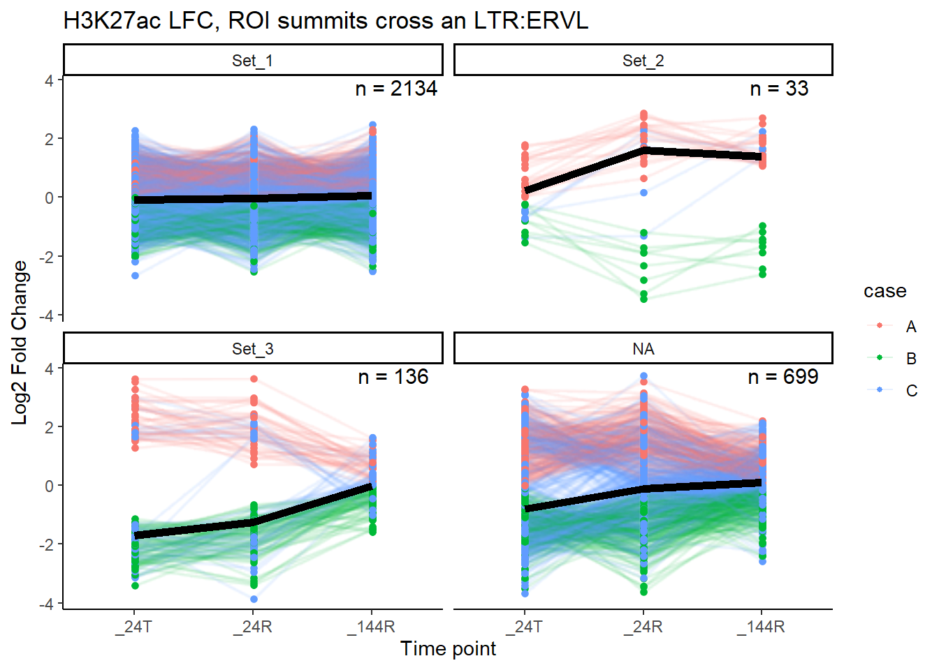

Past versions of "All LTRs and summits ERV1-3.png"

Version	Author	Date
81af285	reneeisnowhere	2026-02-04

median_LFC_H3K27ac_group_plot(K27ac_lfctable,"ERVK")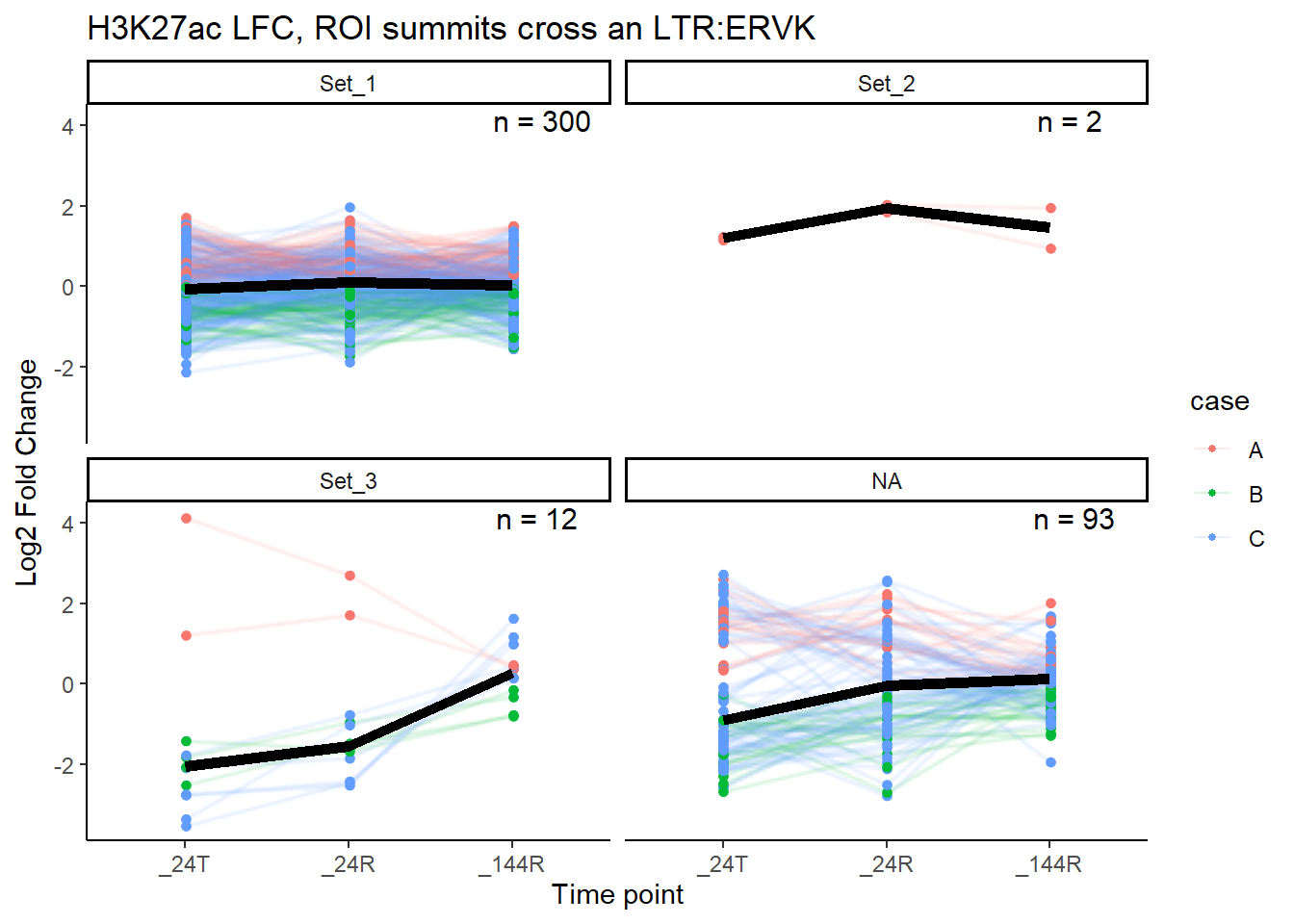

Past versions of "All LTRs and summits ERV1-4.png"

Version	Author	Date
81af285	reneeisnowhere	2026-02-04

median_LFC_H3K27ac_group_plot(K27ac_lfctable,"Gypsy")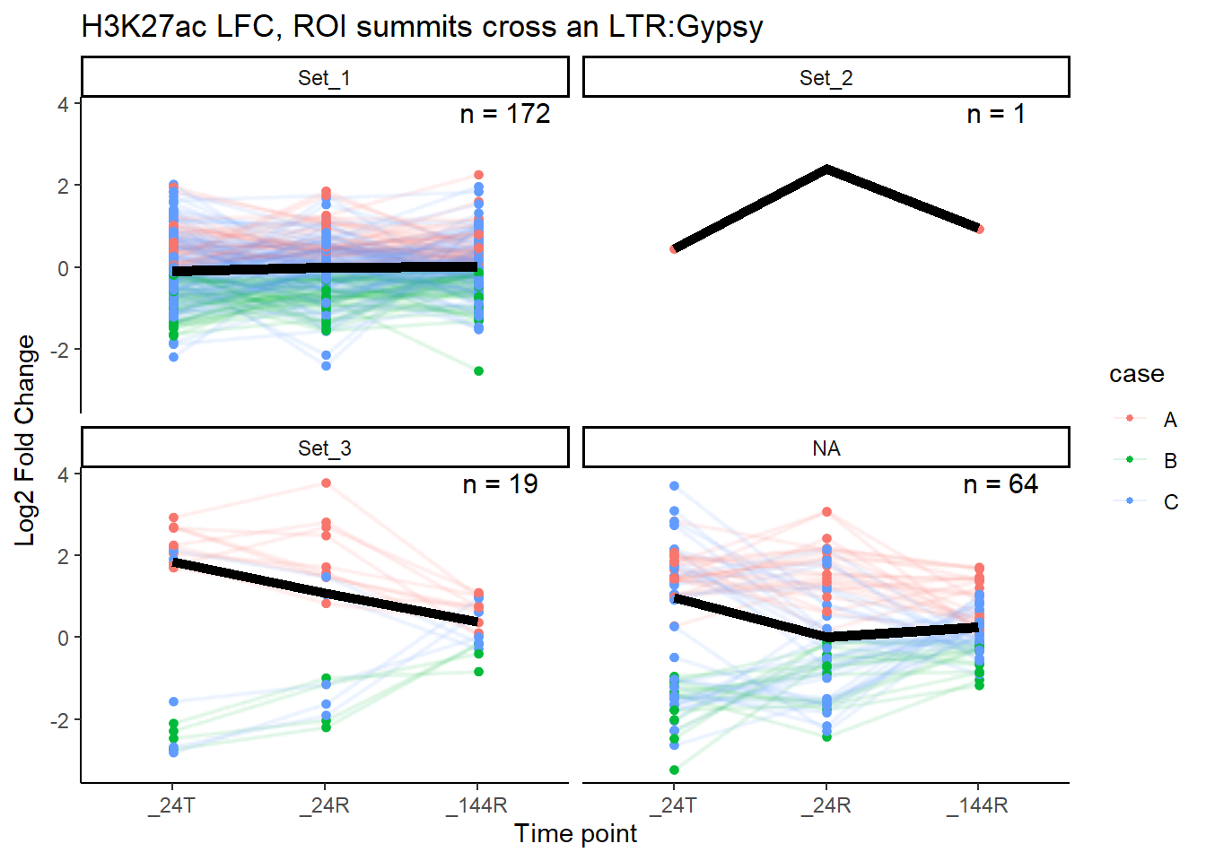

Past versions of "All LTRs and summits ERV1-5.png"

Version	Author	Date
81af285	reneeisnowhere	2026-02-04

median_LFC_H3K27ac_group_plot(K27ac_lfctable,"LTR")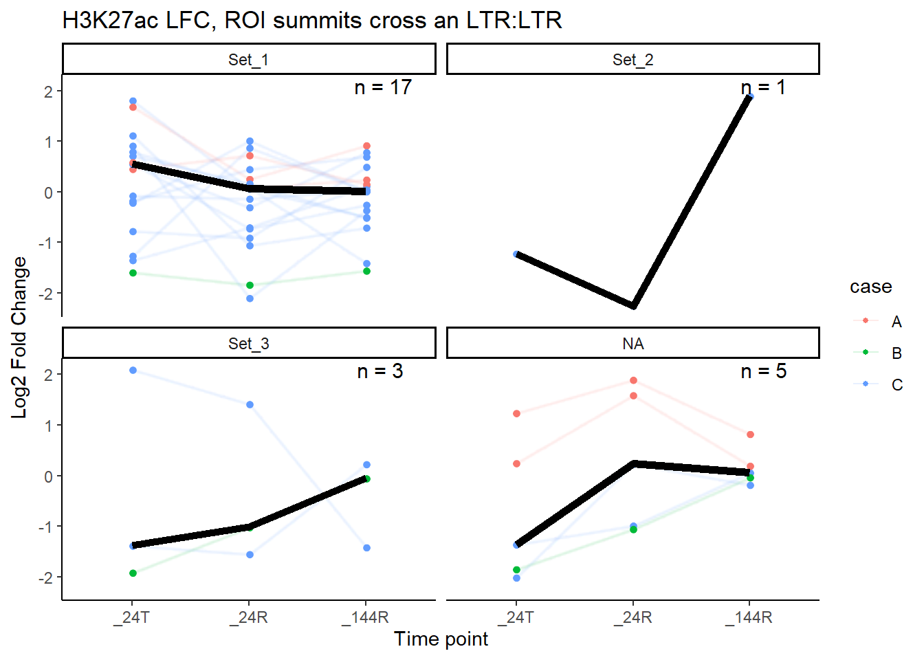

Past versions of "All LTRs and summits ERV1-6.png"

Version	Author	Date
81af285	reneeisnowhere	2026-02-04

Age questions

I had a question about age and LTRs:

age_summit_kw <- LTR_summits_overlap_df %>% 
  left_join(H3K27ac_lookup) %>% 
  filter(cluster %in% c("Set_1","Set_2","Set_3")) %>% 
  group_by(TE_type) %>% 
  summarise(
    kw_p = kruskal.test(milliDiv ~ cluster)$p.value)

age_summit_kw

# A tibble: 6 × 2
  TE_type     kw_p
  <chr>      <dbl>
1 ERV1      0.177 
2 ERVK      0.681 
3 ERVL      0.0257
4 ERVL-MaLR 0.0299
5 Gypsy     0.0835
6 LTR       0.306 

test_TE_age_pairs_summits <- function(df,
                              TE_type_query,
                              sets = c("Set_1", "Set_2", "Set_3")) {

  pid_df <- split_summit_LTR_peakids[[TE_type_query]]
  
  sub_df <- pid_df %>% 
    dplyr::left_join(H3K27ac_lookup) %>%
   
    dplyr::filter(
      TE_type == TE_type_query,
      cluster %in% sets,
      !is.na(milliDiv)
    )

  # Medians first (ground truth)
  med_df <- sub_df %>% 
    dplyr::group_by(cluster) %>% 
    dplyr::summarise(
      median_age = median(milliDiv, na.rm = TRUE),
      n = dplyr::n(),
      .groups = "drop"
    )

  # Pairwise Wilcoxon
  pw <- pairwise.wilcox.test(
    x = sub_df$milliDiv,
    g = sub_df$cluster,
    p.adjust.method = "BH"
  )

  # Tidy + enforce symmetric pairs
  pw_df <- as.data.frame(as.table(pw$p.value)) %>% 
    dplyr::filter(!is.na(Freq)) %>% 
    dplyr::rename(
      set_A = Var1,
      set_B = Var2,
      p_adj = Freq
    )

  # Join medians *by value*, not position
  pw_df %>% 
    dplyr::left_join(med_df, by = c("set_A" = "cluster")) %>% 
    dplyr::rename(median_A = median_age, n_A = n) %>% 
    dplyr::left_join(med_df, by = c("set_B" = "cluster")) %>% 
    dplyr::rename(median_B = median_age, n_B = n) %>% 
    dplyr::mutate(
      older_set = dplyr::case_when(
        median_A > median_B ~ set_A,
        median_B > median_A ~ set_B,
        TRUE ~ "equal"
      ),
      TE_type = TE_type_query
    )
}

testing age pairs between ROI summits

test_TE_age_pairs_summits(LTR_summits_overlap_df, "ERVL")

  set_A set_B      p_adj median_A n_A median_B  n_B older_set TE_type
1 Set_2 Set_1 0.55190415      254  33      244 2137     Set_2    ERVL
2 Set_3 Set_1 0.02482948      256 136      244 2137     Set_3    ERVL
3 Set_3 Set_2 0.55190415      256 136      254   33     Set_3    ERVL

test_TE_age_pairs_summits(LTR_summits_overlap_df, "ERV1")

  set_A set_B     p_adj median_A n_A median_B  n_B older_set TE_type
1 Set_2 Set_1 0.8642775      150  33      156 1837     Set_1    ERV1
2 Set_3 Set_1 0.1945868      150 203      156 1837     Set_1    ERV1
3 Set_3 Set_2 0.6037261      150 203      150   33     equal    ERV1

test_TE_age_pairs_summits(LTR_summits_overlap_df, "ERVL-MaLR")

  set_A set_B     p_adj median_A n_A median_B  n_B older_set   TE_type
1 Set_2 Set_1 0.1007233      247  53      235 2699     Set_2 ERVL-MaLR
2 Set_3 Set_1 0.1455446      246 201      235 2699     Set_3 ERVL-MaLR
3 Set_3 Set_2 0.2753333      246 201      247   53     Set_2 ERVL-MaLR

compare_case_age <- function(df,
                             TE_family,
                             set_case_1,
                             set_case_2) {

  sub_df <- df %>% 
    dplyr::left_join(set_case_list_H3K27ac, by=c("Peakid"="genes")) %>% 
    dplyr::filter(
      TE_type == TE_family,
      set_case %in% c(set_case_1, set_case_2),
      !is.na(milliDiv)
    )

  med_df <- sub_df %>% 
    dplyr::group_by(set_case) %>% 
    dplyr::summarise(
      median_age = median(milliDiv),
      n = dplyr::n(),
      .groups = "drop"
    )

  test <- wilcox.test(milliDiv ~ set_case, data = sub_df)

  tibble::tibble(
    TE_type = TE_family,
    group_1 = set_case_1,
    group_2 = set_case_2,
    median_1 = med_df$median_age[med_df$set_case == set_case_1],
    median_2 = med_df$median_age[med_df$set_case == set_case_2],
    n_1 = med_df$n[med_df$set_case == set_case_1],
    n_2 = med_df$n[med_df$set_case == set_case_2],
    p_value = test$p.value,
    older_group = dplyr::case_when(
      median_1 > median_2 ~ set_case_1,
      median_2 > median_1 ~ set_case_2,
      TRUE ~ "equal"
    )
  )
}

LTR_summits_overlap_df %>% 
  dplyr::left_join(set_case_list_H3K27ac, by=c("Peakid"="genes")) %>%
  dplyr::filter(
    TE_type == "ERV1",
    set_case %in% c("Set_1_A", "Set_2_A")
  ) %>% 
  ggplot(aes(x = set_case, y = milliDiv, fill = set_case)) +
  geom_violin(trim = FALSE) +
  geom_boxplot(width = 0.15, outlier.shape = NA) +
  theme_classic() +
  labs(
    y = "Divergence from consensus (milliDiv)",
    x = NULL,
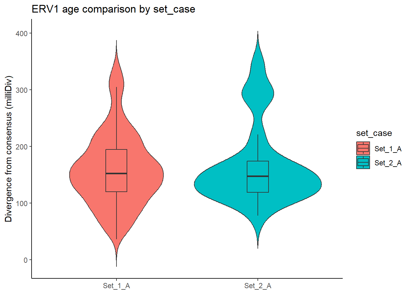
    title = "ERV1 age comparison by set_case"
  )

Past versions of unnamed-chunk-17-1.png

Version	Author	Date
81af285	reneeisnowhere	2026-02-04

compare_case_age(LTR_summits_overlap_df,"ERV1","Set_1_A","Set_3_A")

# A tibble: 1 × 9
  TE_type group_1 group_2 median_1 median_2   n_1   n_2 p_value older_group
  <chr>   <chr>   <chr>      <dbl>    <dbl> <int> <int>   <dbl> <chr>      
1 ERV1    Set_1_A Set_3_A     152.      150   292   115   0.308 Set_1_A    

compare_case_age(LTR_summits_overlap_df,"ERVL","Set_1_A","Set_3_A")

# A tibble: 1 × 9
  TE_type group_1 group_2 median_1 median_2   n_1   n_2 p_value older_group
  <chr>   <chr>   <chr>      <dbl>    <dbl> <int> <int>   <dbl> <chr>      
1 ERVL    Set_1_A Set_3_A      242      221   339    33   0.311 Set_1_A    

compare_case_age(LTR_summits_overlap_df,"ERVK","Set_1_A","Set_3_A")

# A tibble: 1 × 9
  TE_type group_1 group_2 median_1 median_2   n_1   n_2 p_value older_group
  <chr>   <chr>   <chr>      <dbl>    <dbl> <int> <int>   <dbl> <chr>      
1 ERVK    Set_1_A Set_3_A     87.5       82    60     2   0.780 Set_1_A    

compare_case_age(LTR_summits_overlap_df,"ERVL-MaLR","Set_1_A","Set_3_A")

# A tibble: 1 × 9
  TE_type   group_1 group_2 median_1 median_2   n_1   n_2 p_value older_group
  <chr>     <chr>   <chr>      <dbl>    <dbl> <int> <int>   <dbl> <chr>      
1 ERVL-MaLR Set_1_A Set_3_A      237      244   477    71   0.548 Set_3_A    

compare_case_age(LTR_summits_overlap_df,"ERV1","Set_1_A","Set_3_A")

# A tibble: 1 × 9
  TE_type group_1 group_2 median_1 median_2   n_1   n_2 p_value older_group
  <chr>   <chr>   <chr>      <dbl>    <dbl> <int> <int>   <dbl> <chr>      
1 ERV1    Set_1_A Set_3_A     152.      150   292   115   0.308 Set_1_A    

compare_case_age(LTR_summits_overlap_df,"ERV1","Set_1_A","Set_3_A")

# A tibble: 1 × 9
  TE_type group_1 group_2 median_1 median_2   n_1   n_2 p_value older_group
  <chr>   <chr>   <chr>      <dbl>    <dbl> <int> <int>   <dbl> <chr>      
1 ERV1    Set_1_A Set_3_A     152.      150   292   115   0.308 Set_1_A    

ERV1_summit_df <- split_summit_LTR_peakids$ERV1 %>% 
  left_join(., set_case_list_H3K27ac, by = c("Peakid"="genes")) %>% 
  dplyr::filter(cluster %in% c("Set_1","Set_2","Set_3"))  
  

cluster_pairs <- list(c("Set_1","Set_2"),
                      c("Set_1", "Set_3"),
                      c("Set_2","Set_3"))


ERV1_pval_df <- ERV1_summit_df %>%
  group_by(case) %>%
  group_modify(~ {
    map_dfr(cluster_pairs, function(pair) {
      x <- .x %>% filter(cluster == pair[1]) %>% pull(milliDiv)
      y <- .x %>% filter(cluster == pair[2]) %>% pull(milliDiv)
      tibble(
        cluster1 = pair[1],
        cluster2 = pair[2],
        p_value = wilcox.test(x, y)$p.value)
    })
  })


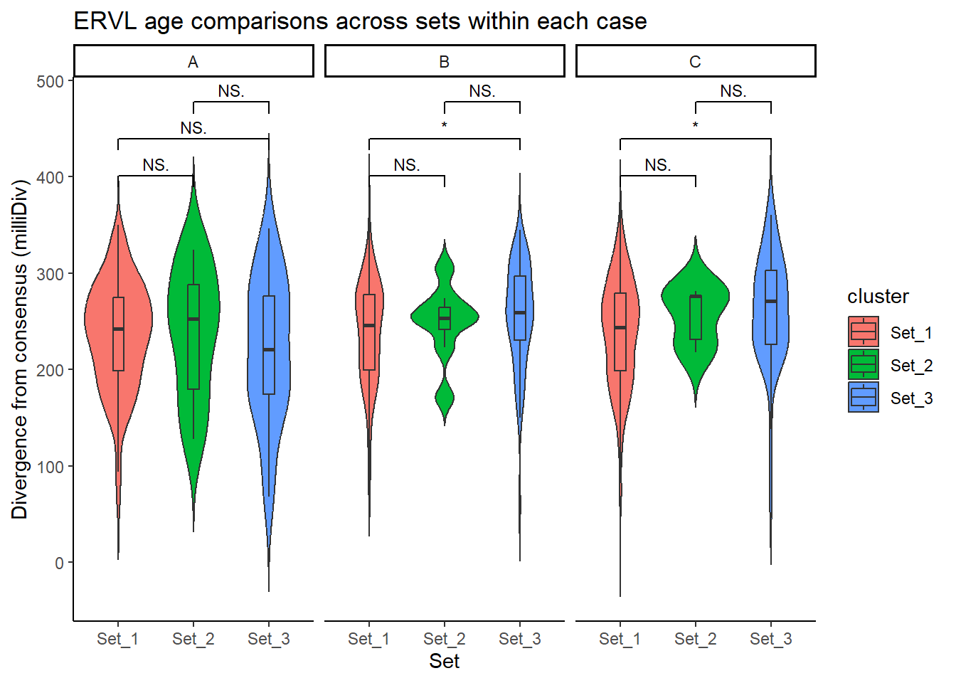
ggplot(ERV1_summit_df, aes(x = cluster, y = milliDiv, fill = cluster)) +
  geom_violin(trim = FALSE) +
  geom_boxplot(width = 0.15, outlier.shape = NA) +
  facet_wrap(~case) +
  theme_classic() +
  labs(
    y = "Divergence from consensus (milliDiv)",
    x = "Set",
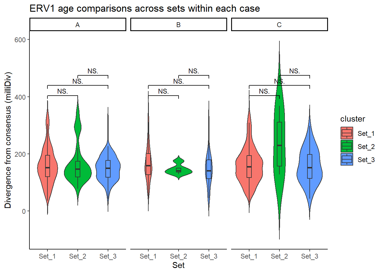
    title = "ERV1 age comparisons across sets within each case"
  ) +
  geom_signif(
    comparisons = cluster_pairs,
    test = "wilcox.test",
    map_signif_level = TRUE,
    textsize = 3,
    step_increase = 0.1
  )

Past versions of "ERV1 case summit-1.png"

Version	Author	Date
81af285	reneeisnowhere	2026-02-04

ERVL_summit_df <- split_summit_LTR_peakids$ERVL %>% 
  left_join(., set_case_list_H3K27ac, by = c("Peakid"="genes")) %>% 
  dplyr::filter(cluster %in% c("Set_1","Set_2","Set_3"))  
  

cluster_pairs <- list(c("Set_1","Set_2"),
                      c("Set_1", "Set_3"),
                      c("Set_2","Set_3"))


ERVL_pval_df <- ERVL_summit_df %>%
  group_by(case) %>%
  group_modify(~ {
    map_dfr(cluster_pairs, function(pair) {
      x <- .x %>% filter(cluster == pair[1]) %>% pull(milliDiv)
      y <- .x %>% filter(cluster == pair[2]) %>% pull(milliDiv)
      tibble(
        cluster1 = pair[1],
        cluster2 = pair[2],
        p_value = wilcox.test(x, y)$p.value)
    })
  })


ggplot(ERVL_summit_df, aes(x = cluster, y = milliDiv, fill = cluster)) +
  geom_violin(trim = FALSE) +
  geom_boxplot(width = 0.15, outlier.shape = NA) +
  facet_wrap(~case) +
  theme_classic() +
  labs(
    y = "Divergence from consensus (milliDiv)",
    x = "Set",
    title = "ERVL age comparisons across sets within each case"
  ) +
  geom_signif(
    comparisons = cluster_pairs,
    test = "wilcox.test",
    map_signif_level = TRUE,
    textsize = 3,
    step_increase = 0.1
  )

Past versions of "ERVL case summit-1.png"

Version	Author	Date
81af285	reneeisnowhere	2026-02-04

split_summit_LTR_peakids$ERV1 %>% 
  left_join(., set_case_list_H3K27ac, by = c("Peakid"="genes")) %>% 
  dplyr::filter(cluster %in% c("Set_1","Set_2","Set_3")) %>% 
  ggplot(., aes(x = cluster, y = milliDiv)) +
  geom_violin(trim = FALSE) +
   geom_boxplot(width = 0.15, outlier.shape = NA) +
  facet_wrap(~case)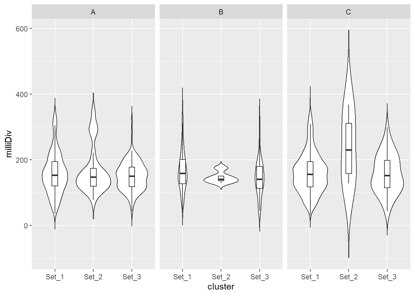

Past versions of unnamed-chunk-19-1.png

Version	Author	Date
81af285	reneeisnowhere	2026-02-04

ERV1_case_df <- split_summit_LTR_peakids$ERV1 %>% 
  left_join(set_case_list_H3K27ac, by = c("Peakid" = "genes")) %>% 
  filter(cluster %in% c("Set_1", "Set_2", "Set_3"),
         case %in% c("A", "B"))  # only compare A vs B


ggplot(ERV1_case_df, aes(x = case, y = milliDiv, fill = case)) +
  geom_violin(trim = FALSE) +
  geom_boxplot(width = 0.15, outlier.shape = NA) +
  facet_wrap(~cluster) +
  theme_classic() +
  labs(
    y = "Divergence from consensus (milliDiv)",
    x = "Case",
    title = "ERV1 age comparison: A vs B within each cluster"
  ) +
  geom_signif(
    comparisons = list(c("A", "B")),
    test = "wilcox.test",
    map_signif_level = TRUE,
    textsize = 3,
    step_increase = .1)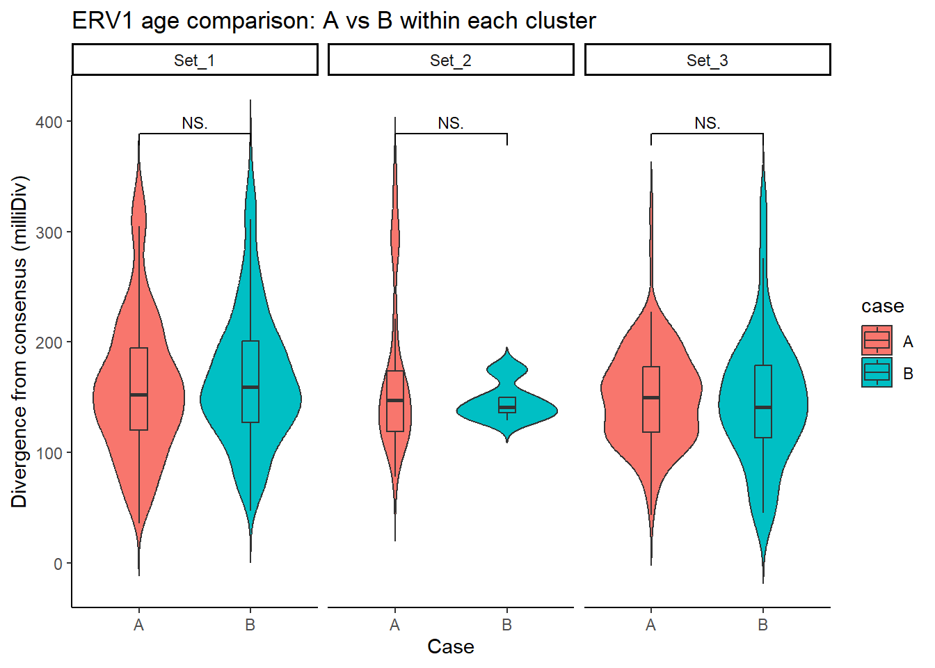

Past versions of "ERV1 case plot-1.png"

Version	Author	Date
81af285	reneeisnowhere	2026-02-04

ERVL_case_df <- split_summit_LTR_peakids$ERVL %>% 
  left_join(set_case_list_H3K27ac, by = c("Peakid" = "genes")) %>% 
  filter(cluster %in% c("Set_1", "Set_2", "Set_3"),
         case %in% c("A", "B"))  # only compare A vs B


ggplot(ERVL_case_df, aes(x = case, y = milliDiv, fill = case)) +
  geom_violin(trim = FALSE) +
  geom_boxplot(width = 0.15, outlier.shape = NA) +
  facet_wrap(~cluster) +
  theme_classic() +
  labs(
    y = "Divergence from consensus (milliDiv)",
    x = "Case",
    title = "ERVL age comparison: A vs B within each cluster"
  ) +
  geom_signif(
    comparisons = list(c("A", "B")),
    test = "wilcox.test",
    map_signif_level = TRUE,
    textsize = 3,
    step_increase = .1)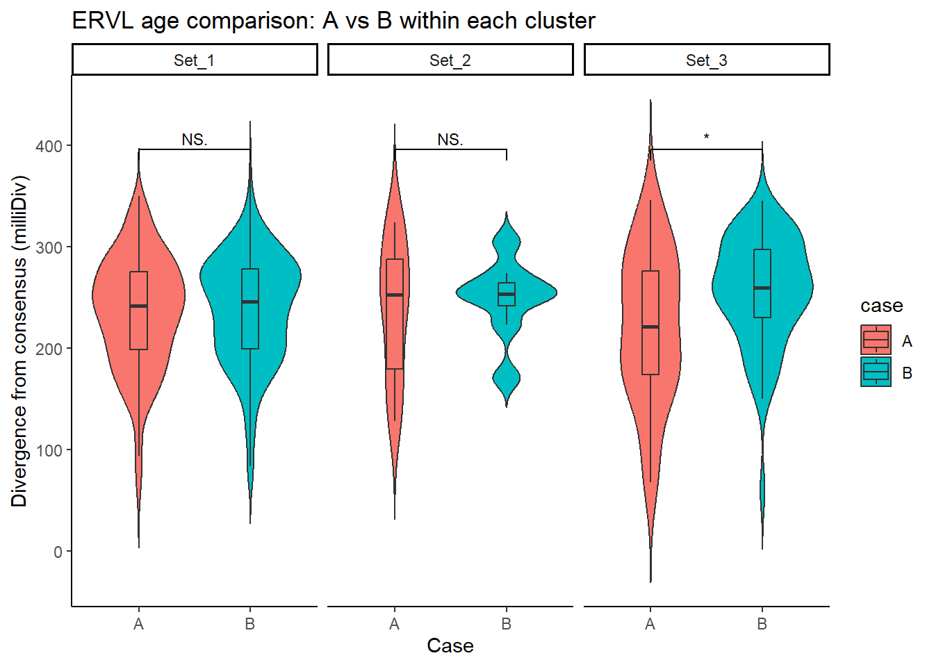

Past versions of "ERVL case plot-1.png"

Version	Author	Date
81af285	reneeisnowhere	2026-02-04

ERVK_case_df <- split_summit_LTR_peakids$ERVK %>% 
  left_join(set_case_list_H3K27ac, by = c("Peakid" = "genes")) %>% 
  filter(cluster %in% c("Set_1", "Set_2", "Set_3"),
         case %in% c("A", "B"))  # only compare A vs B


ggplot(ERVK_case_df, aes(x = case, y = milliDiv, fill = case)) +
  geom_violin(trim = FALSE) +
  geom_boxplot(width = 0.15, outlier.shape = NA) +
  facet_wrap(~cluster) +
  theme_classic() +
  labs(
    y = "Divergence from consensus (milliDiv)",
    x = "Case",
    title = "ERVK age comparison: A vs B within each cluster"
  ) +
  geom_signif(
    comparisons = list(c("A", "B")),
    test = "wilcox.test",
    map_signif_level = TRUE,
    textsize = 3,
    step_increase = .1)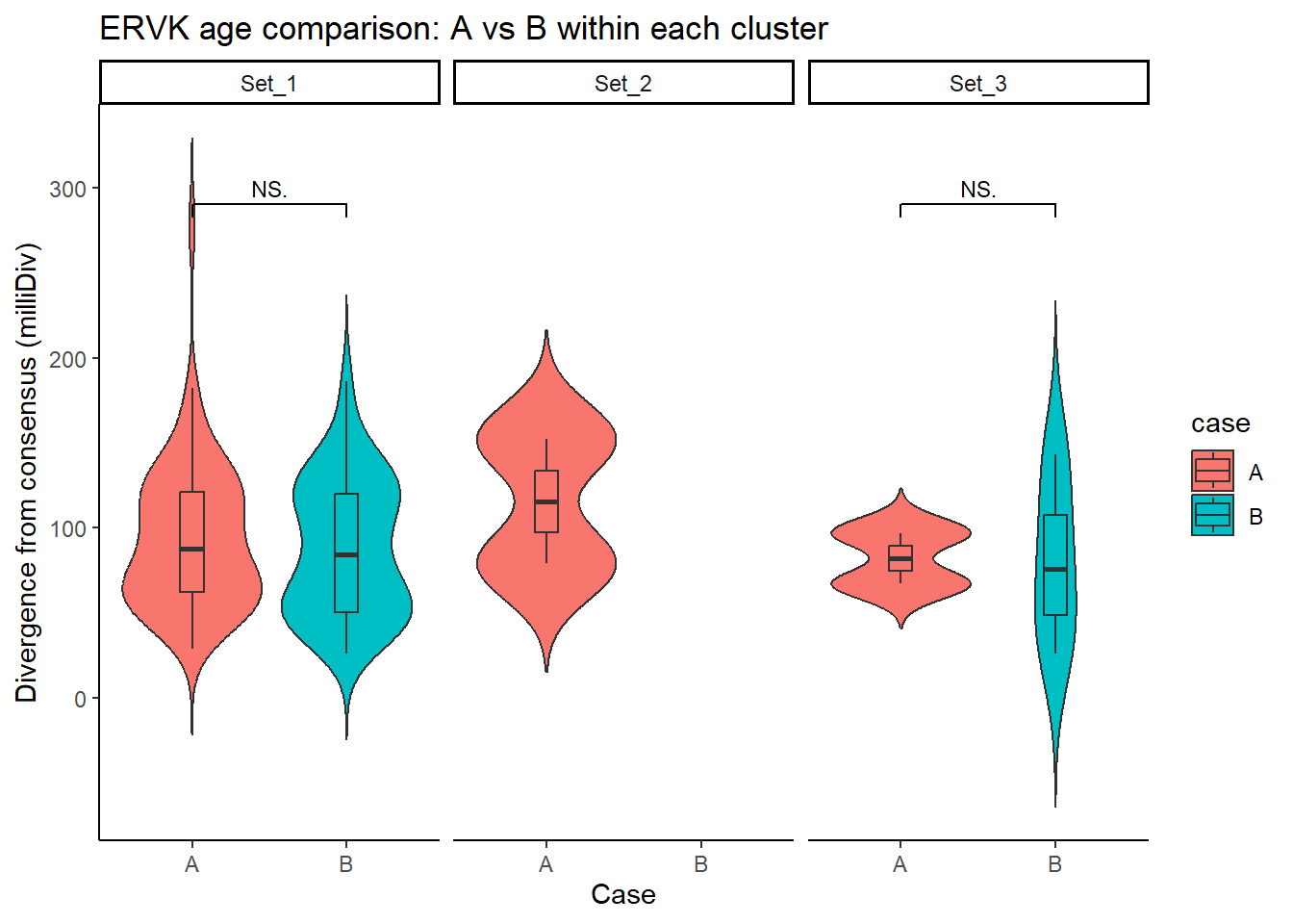

Past versions of "ERVK case plot-1.png"

Version	Author	Date
81af285	reneeisnowhere	2026-02-04

ERVL_MaLR_case_df <- split_summit_LTR_peakids$`ERVL-MaLR` %>% 
  left_join(set_case_list_H3K27ac, by = c("Peakid" = "genes")) %>% 
  filter(cluster %in% c("Set_1", "Set_2", "Set_3"),
         case %in% c("A", "B"))  # only compare A vs B


ggplot(ERVL_MaLR_case_df, aes(x = case, y = milliDiv, fill = case)) +
  geom_violin(trim = FALSE) +
  geom_boxplot(width = 0.15, outlier.shape = NA) +
  facet_wrap(~cluster) +
  theme_classic() +
  labs(
    y = "Divergence from consensus (milliDiv)",
    x = "Case",
    title = "ERVL-MaLR age comparison: A vs B within each cluster"
  ) +
  geom_signif(
    comparisons = list(c("A", "B")),
    test = "wilcox.test",
    map_signif_level = TRUE,
    textsize = 3,
    step_increase = .1)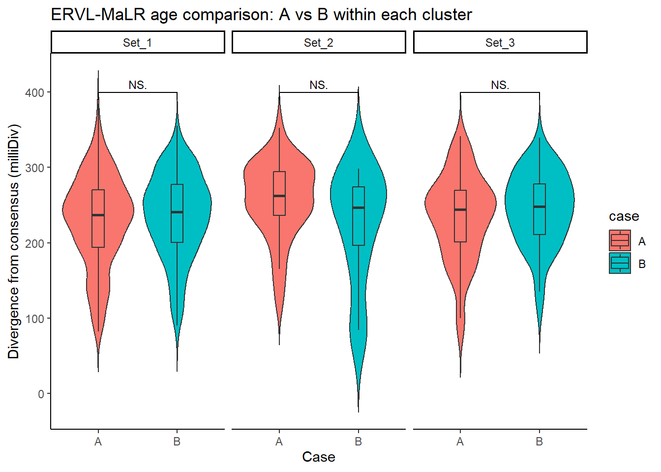

Past versions of "ERVL-MaLR case plot-1.png"

Version	Author	Date
81af285	reneeisnowhere	2026-02-04

Gypsy_case_df <- split_summit_LTR_peakids$Gypsy %>% 
  left_join(set_case_list_H3K27ac, by = c("Peakid" = "genes")) %>% 
  filter(cluster %in% c("Set_1", "Set_2", "Set_3"),
         case %in% c("A", "B"))  # only compare A vs B


ggplot(Gypsy_case_df, aes(x = case, y = milliDiv, fill = case)) +
  geom_violin(trim = FALSE) +
  geom_boxplot(width = 0.15, outlier.shape = NA) +
  facet_wrap(~cluster) +
  theme_classic() +
  labs(
    y = "Divergence from consensus (milliDiv)",
    x = "Case",
    title = "Gypsy age comparison: A vs B within each cluster"
  ) +
  geom_signif(
    comparisons = list(c("A", "B")),
    test = "wilcox.test",
    map_signif_level = TRUE,
    textsize = 3,
    step_increase = .1)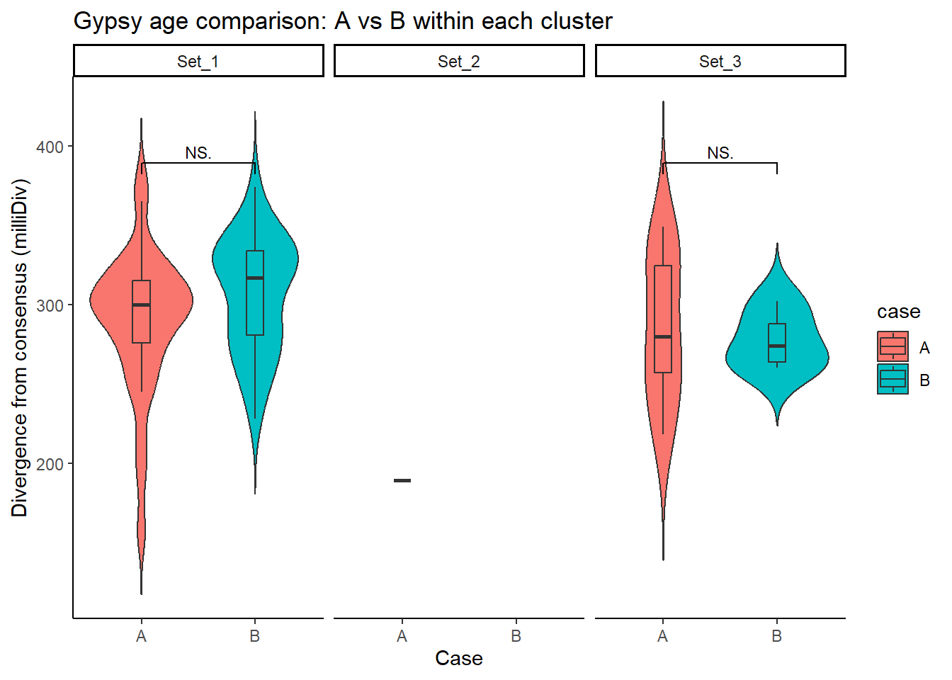

Past versions of "Gypsy case plot-1.png"

Version	Author	Date
81af285	reneeisnowhere	2026-02-04

LTR_case_df <- split_summit_LTR_peakids$LTR %>% 
  left_join(set_case_list_H3K27ac, by = c("Peakid" = "genes")) %>% 
  filter(cluster %in% c("Set_1", "Set_2", "Set_3"),
         case %in% c("A", "B"))  # only compare A vs B


ggplot(LTR_case_df, aes(x = case, y = milliDiv, fill = case)) +
  geom_violin(trim = FALSE) +
  geom_boxplot(width = 0.15, outlier.shape = NA) +
  facet_wrap(~cluster) +
  theme_classic() +
  labs(
    y = "Divergence from consensus (milliDiv)",
    x = "Case",
    title = "LTR age comparison: A vs B within each cluster"
  ) +
  geom_signif(
    comparisons = list(c("A", "B")),
    test = "wilcox.test",
    map_signif_level = TRUE,
    textsize = 3,
    step_increase = .1)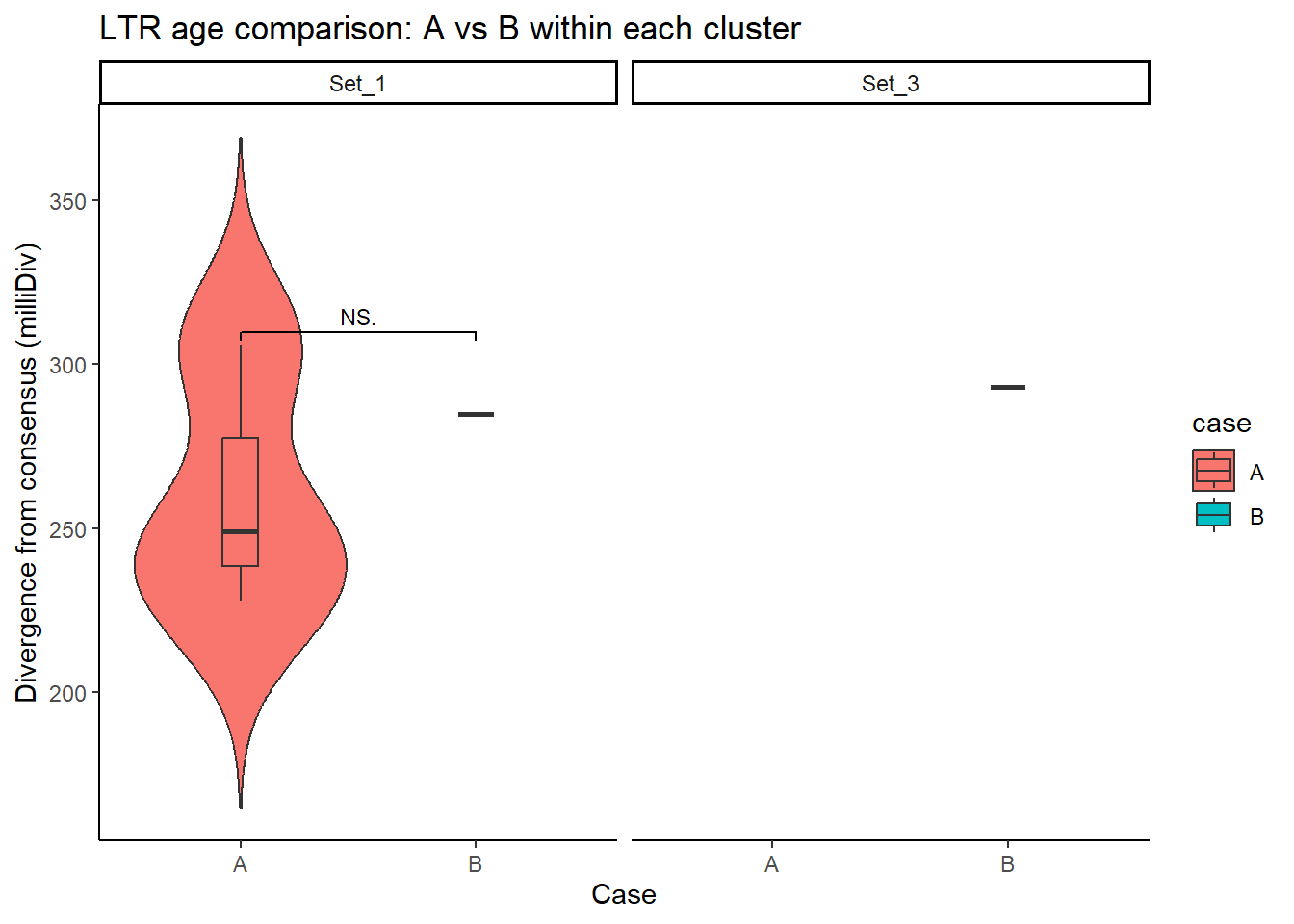

Past versions of "LTR case plot-1.png"

Version	Author	Date
81af285	reneeisnowhere	2026-02-04

listit <- data.frame(x=width(H3K9me3_sets_gr$all_H3K9me3_regions))
ggplot(listit, aes(x=x))+
  geom_density()+ggtitle("H3K9me3 ROI widths")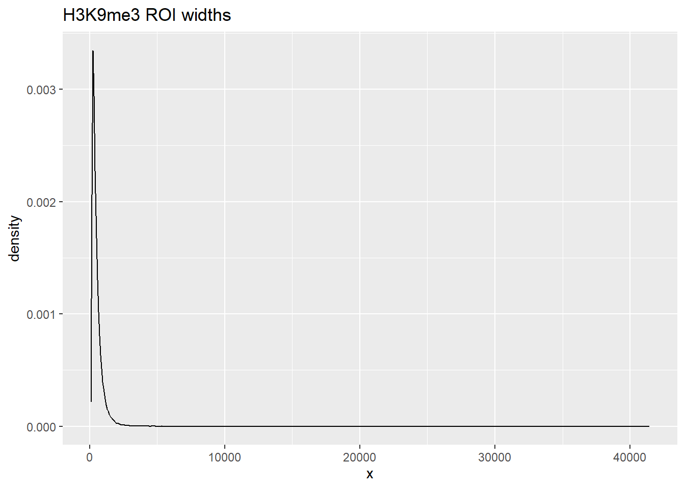

Past versions of unnamed-chunk-20-1.png

Version	Author	Date
3a5cba8	reneeisnowhere	2026-02-06
81af285	reneeisnowhere	2026-02-04

listit_k27ac <- data.frame(x=width(H3K27ac_sets_gr$all_H3K27ac))

listit %>% 
  summary()

       x          
 Min.   :   85.0  
 1st Qu.:  264.0  
 Median :  394.0  
 Mean   :  519.2  
 3rd Qu.:  634.0  
 Max.   :41434.0  

ggplot(listit_k27ac, aes(x=x))+
  geom_density()+ggtitle("H3K27ac ROI widths")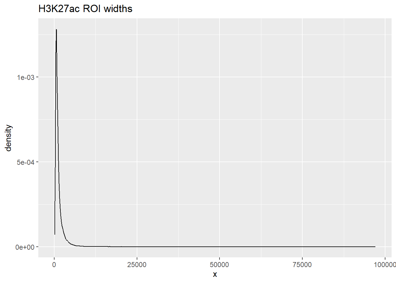

Past versions of unnamed-chunk-20-2.png

Version	Author	Date
3a5cba8	reneeisnowhere	2026-02-06
81af285	reneeisnowhere	2026-02-04

listit_k27ac %>% 
  summary()

       x        
 Min.   :   87  
 1st Qu.:  581  
 Median :  869  
 Mean   : 1299  
 3rd Qu.: 1469  
 Max.   :97107  

Session information

sessionInfo()

R version 4.4.2 (2024-10-31 ucrt)
Platform: x86_64-w64-mingw32/x64
Running under: Windows 11 x64 (build 26200)

Matrix products: default


locale:
[1] LC_COLLATE=English_United States.utf8 
[2] LC_CTYPE=English_United States.utf8   
[3] LC_MONETARY=English_United States.utf8
[4] LC_NUMERIC=C                          
[5] LC_TIME=English_United States.utf8    

time zone: America/Chicago
tzcode source: internal

attached base packages:
[1] grid      stats4    stats     graphics  grDevices utils     datasets 
[8] methods   base     

other attached packages:
 [1] ggsignif_0.6.4       smplot2_0.2.5        ggVennDiagram_1.5.4 
 [4] ChIPseeker_1.42.1    DT_0.33              ggrepel_0.9.6       
 [7] rtracklayer_1.66.0   genomation_1.38.0    plyranges_1.26.0    
[10] GenomicRanges_1.58.0 GenomeInfoDb_1.42.3  IRanges_2.40.1      
[13] S4Vectors_0.44.0     BiocGenerics_0.52.0  lubridate_1.9.4     
[16] forcats_1.0.0        stringr_1.5.1        dplyr_1.1.4         
[19] purrr_1.1.0          readr_2.1.5          tidyr_1.3.1         
[22] tibble_3.3.0         ggplot2_3.5.2        tidyverse_2.0.0     
[25] workflowr_1.7.1     

loaded via a namespace (and not attached):
  [1] splines_4.4.2                          
  [2] later_1.4.2                            
  [3] BiocIO_1.16.0                          
  [4] bitops_1.0-9                           
  [5] ggplotify_0.1.2                        
  [6] R.oo_1.27.1                            
  [7] XML_3.99-0.18                          
  [8] rpart_4.1.24                           
  [9] lifecycle_1.0.4                        
 [10] rstatix_0.7.2                          
 [11] rprojroot_2.1.1                        
 [12] vroom_1.6.5                            
 [13] processx_3.8.6                         
 [14] lattice_0.22-7                         
 [15] crosstalk_1.2.2                        
 [16] backports_1.5.0                        
 [17] magrittr_2.0.3                         
 [18] Hmisc_5.2-3                            
 [19] sass_0.4.10                            
 [20] rmarkdown_2.29                         
 [21] jquerylib_0.1.4                        
 [22] yaml_2.3.10                            
 [23] plotrix_3.8-4                          
 [24] httpuv_1.6.16                          
 [25] ggtangle_0.0.7                         
 [26] cowplot_1.2.0                          
 [27] DBI_1.2.3                              
 [28] RColorBrewer_1.1-3                     
 [29] abind_1.4-8                            
 [30] zlibbioc_1.52.0                        
 [31] R.utils_2.13.0                         
 [32] RCurl_1.98-1.17                        
 [33] yulab.utils_0.2.1                      
 [34] nnet_7.3-20                            
 [35] rappdirs_0.3.3                         
 [36] git2r_0.36.2                           
 [37] GenomeInfoDbData_1.2.13                
 [38] enrichplot_1.26.6                      
 [39] tidytree_0.4.6                         
 [40] codetools_0.2-20                       
 [41] DelayedArray_0.32.0                    
 [42] DOSE_4.0.1                             
 [43] tidyselect_1.2.1                       
 [44] aplot_0.2.8                            
 [45] UCSC.utils_1.2.0                       
 [46] farver_2.1.2                           
 [47] matrixStats_1.5.0                      
 [48] base64enc_0.1-3                        
 [49] GenomicAlignments_1.42.0               
 [50] jsonlite_2.0.0                         
 [51] Formula_1.2-5                          
 [52] tools_4.4.2                            
 [53] treeio_1.30.0                          
 [54] TxDb.Hsapiens.UCSC.hg19.knownGene_3.2.2
 [55] Rcpp_1.1.0                             
 [56] glue_1.8.0                             
 [57] gridExtra_2.3                          
 [58] SparseArray_1.6.2                      
 [59] xfun_0.52                              
 [60] qvalue_2.38.0                          
 [61] MatrixGenerics_1.18.1                  
 [62] withr_3.0.2                            
 [63] fastmap_1.2.0                          
 [64] boot_1.3-32                            
 [65] callr_3.7.6                            
 [66] caTools_1.18.3                         
 [67] digest_0.6.37                          
 [68] timechange_0.3.0                       
 [69] R6_2.6.1                               
 [70] gridGraphics_0.5-1                     
 [71] seqPattern_1.38.0                      
 [72] colorspace_2.1-1                       
 [73] Cairo_1.6-5                            
 [74] GO.db_3.20.0                           
 [75] gtools_3.9.5                           
 [76] dichromat_2.0-0.1                      
 [77] RSQLite_2.4.3                          
 [78] R.methodsS3_1.8.2                      
 [79] utf8_1.2.6                             
 [80] generics_0.1.4                         
 [81] data.table_1.17.8                      
 [82] httr_1.4.7                             
 [83] htmlwidgets_1.6.4                      
 [84] S4Arrays_1.6.0                         
 [85] whisker_0.4.1                          
 [86] pkgconfig_2.0.3                        
 [87] gtable_0.3.6                           
 [88] blob_1.2.4                             
 [89] impute_1.80.0                          
 [90] XVector_0.46.0                         
 [91] htmltools_0.5.8.1                      
 [92] carData_3.0-5                          
 [93] pwr_1.3-0                              
 [94] fgsea_1.32.4                           
 [95] scales_1.4.0                           
 [96] Biobase_2.66.0                         
 [97] png_0.1-8                              
 [98] ggfun_0.2.0                            
 [99] knitr_1.50                             
[100] rstudioapi_0.17.1                      
[101] tzdb_0.5.0                             
[102] reshape2_1.4.4                         
[103] rjson_0.2.23                           
[104] checkmate_2.3.3                        
[105] nlme_3.1-168                           
[106] curl_7.0.0                             
[107] zoo_1.8-14                             
[108] cachem_1.1.0                           
[109] KernSmooth_2.23-26                     
[110] vipor_0.4.7                            
[111] parallel_4.4.2                         
[112] foreign_0.8-90                         
[113] AnnotationDbi_1.68.0                   
[114] ggrastr_1.0.2                          
[115] restfulr_0.0.16                        
[116] pillar_1.11.0                          
[117] vctrs_0.6.5                            
[118] gplots_3.2.0                           
[119] ggpubr_0.6.1                           
[120] promises_1.3.3                         
[121] car_3.1-3                              
[122] cluster_2.1.8.1                        
[123] beeswarm_0.4.0                         
[124] htmlTable_2.4.3                        
[125] evaluate_1.0.5                         
[126] GenomicFeatures_1.58.0                 
[127] cli_3.6.5                              
[128] compiler_4.4.2                         
[129] Rsamtools_2.22.0                       
[130] rlang_1.1.6                            
[131] crayon_1.5.3                           
[132] labeling_0.4.3                         
[133] ps_1.9.1                               
[134] ggbeeswarm_0.7.2                       
[135] getPass_0.2-4                          
[136] plyr_1.8.9                             
[137] fs_1.6.6                               
[138] stringi_1.8.7                          
[139] gridBase_0.4-7                         
[140] BiocParallel_1.40.2                    
[141] Biostrings_2.74.1                      
[142] lazyeval_0.2.2                         
[143] GOSemSim_2.32.0                        
[144] Matrix_1.7-3                           
[145] BSgenome_1.74.0                        
[146] hms_1.1.3                              
[147] patchwork_1.3.2                        
[148] bit64_4.6.0-1                          
[149] KEGGREST_1.46.0                        
[150] SummarizedExperiment_1.36.0            
[151] broom_1.0.9                            
[152] igraph_2.1.4                           
[153] memoise_2.0.1                          
[154] bslib_0.9.0                            
[155] ggtree_3.14.0                          
[156] fastmatch_1.1-6                        
[157] bit_4.6.0                              
[158] ape_5.8-1