CX-revision

workflowr

• Summary
• Checks
• Past versions

Last updated: 2025-11-03

Checks: 7 0

Knit directory: CX_revison/

This reproducible R Markdown analysis was created with workflowr (version 1.7.1). The Checks tab describes the reproducibility checks that were applied when the results were created. The Past versions tab lists the development history.

---

R Markdown file: up-to-date

Great! Since the R Markdown file has been committed to the Git repository, you know the exact version of the code that produced these results.

Environment: empty

Great job! The global environment was empty. Objects defined in the global environment can affect the analysis in your R Markdown file in unknown ways. For reproduciblity it’s best to always run the code in an empty environment.

Seed: set.seed(20251031)

The command set.seed(20251031) was run prior to running the code in the R Markdown file. Setting a seed ensures that any results that rely on randomness, e.g. subsampling or permutations, are reproducible.

Session information: recorded

Great job! Recording the operating system, R version, and package versions is critical for reproducibility.

Cache: none

Nice! There were no cached chunks for this analysis, so you can be confident that you successfully produced the results during this run.

File paths: relative

Great job! Using relative paths to the files within your workflowr project makes it easier to run your code on other machines.

Repository version: d642f3e

Great! You are using Git for version control. Tracking code development and connecting the code version to the results is critical for reproducibility.

The results in this page were generated with repository version d642f3e. See the Past versions tab to see a history of the changes made to the R Markdown and HTML files.

Note that you need to be careful to ensure that all relevant files for the analysis have been committed to Git prior to generating the results (you can use wflow_publish or wflow_git_commit). workflowr only checks the R Markdown file, but you know if there are other scripts or data files that it depends on. Below is the status of the Git repository when the results were generated:

Ignored files:
    Ignored:    .RData
    Ignored:    .Rhistory
    Ignored:    .Rproj.user/

Unstaged changes:
    Modified:   CX_revison.Rproj

Note that any generated files, e.g. HTML, png, CSS, etc., are not included in this status report because it is ok for generated content to have uncommitted changes.

---

These are the previous versions of the repository in which changes were made to the R Markdown (analysis/CX-revision.Rmd) and HTML (docs/CX-revision.html) files. If you’ve configured a remote Git repository (see ?wflow_git_remote), click on the hyperlinks in the table below to view the files as they were in that past version.

File	Version	Author	Date	Message
Rmd	d642f3e	reneeisnowhere	2025-11-03	wflow_publish("analysis/CX-revision.Rmd")
html	f31ecb6	reneeisnowhere	2025-10-31	Build site.
Rmd	45f92fd	reneeisnowhere	2025-10-31	update links
html	10b921a	reneeisnowhere	2025-10-31	Build site.
Rmd	9928965	reneeisnowhere	2025-10-31	updated
html	f2ba629	reneeisnowhere	2025-10-31	Build site.
Rmd	635aef2	reneeisnowhere	2025-10-31	wflow_publish("analysis/CX-revision.Rmd")

---

library(tidyverse)
library(readxl)
library(readr)
library(drc)

adding input data

X87_1_0hr_ipsc_96wellplate_baseline_no_treatment_10_14_2025_251014 <- read_excel("data/Presto_blue_results/87-1_0hr_ipsc_96wellplate_baseline_no_treatment_10-14-2025_251014.xls", 
    skip = 34)

X87_1_48hr_ipsc_96wellplate_CX_DOX_Veh_10_16_2025_251016 <- read_excel("data/Presto_blue_results/87-1_48hr_ipsc_96wellplate_CX-DOX-Veh_10-16-2025_251016.xls", 
    skip = 34)

combo_time_data <- 
X87_1_0hr_ipsc_96wellplate_baseline_no_treatment_10_14_2025_251014 %>% 
  dplyr::filter(Well=="Read 2:560,590") %>% 
  mutate(Well="zero") %>% 
  bind_rows(X87_1_48hr_ipsc_96wellplate_CX_DOX_Veh_10_16_2025_251016 %>% 
              dplyr::filter(Well=="Read 2:560,590") %>% mutate(Well="two_day")) %>% 
  dplyr::rename("Time"=Well) %>% 
  pivot_longer(., A1:H12, names_to = "Well", values_to = "reading") %>% 
  pivot_wider(id_cols=c("Well"), names_from = "Time", values_from = "reading")

Plate_map <- read_excel("data/Presto_blue_results/Plate_map.xlsx")

  base_df <- Plate_map %>%
  pivot_longer(cols = everything(), names_to = "Well") %>%
  separate(col = value, into = c("trt", "conc"), sep = "_") %>%
  left_join(., combo_time_data, by = "Well") %>%
    pivot_longer(cols = c(zero, two_day), names_to = "Time") %>%
  mutate(
    trt  = factor(trt, levels = c("CX", "DOX", "VEH", "Unt", "blank")),   # check these levels match your data
    conc = factor(conc, levels = c("0","0.1","0.5","1","5","10","50","blank")),
    Time = factor(Time, levels = c("zero","two_day"))
  )
  
  # 1. subtract blank per Time and clip negatives
processed <- base_df %>%
  group_by(Time) %>%
  mutate(
    blank_mean = mean(value[trt == "blank"], na.rm = TRUE),
    adj_reading = pmax(value - blank_mean, 0)
  ) %>%
  ungroup()


untx_per_ct <- processed %>%
  filter(trt == "Unt") %>%                 # only VEH rows
  group_by(conc, Time) %>%
  summarise(
    unt_mean = mean(adj_reading, na.rm = TRUE),
    n_unt = n(),
    .groups = "drop"
  )

with_veh <-processed %>%
  left_join(untx_per_ct, by = c( "Time")) %>%
  mutate(
    norm_to_veh = case_when(
      is.na(unt_mean)          ~ NA_real_,               # no VEH present for that conc×Time
      unt_mean == 0            ~ NA_real_,               # avoid division by zero
      TRUE                     ~ (adj_reading / unt_mean) * 100
    )
  )
  
wide_norm <-
with_veh %>%
  dplyr::select(Well, trt, conc.x, Time, norm_to_veh) %>%
  pivot_wider(id_cols = c(Well, trt, conc.x), names_from = Time, values_from = norm_to_veh)
  
  # Step 5: compute between-time ratio (two_day relative to zero) safely
final_df <- wide_norm %>%
  mutate(
    hr_norm = case_when(
      is.na(zero) | is.na(two_day) ~ NA_real_,
      zero == 0                    ~ NA_real_,   # choose NA to flag unreliable ratio (or 0 if you prefer)
      TRUE                         ~ (two_day / zero) * 100
    )
  ) %>%
  filter(trt != "blank")

final_df %>% 
  dplyr::rename("conc"=conc.x) %>% 
  ggplot(., aes(x=conc, y=zero))+
  geom_boxplot(aes(fill=trt))+
  theme_bw()+
  ggtitle("Box plot of normalized day zero across treatments")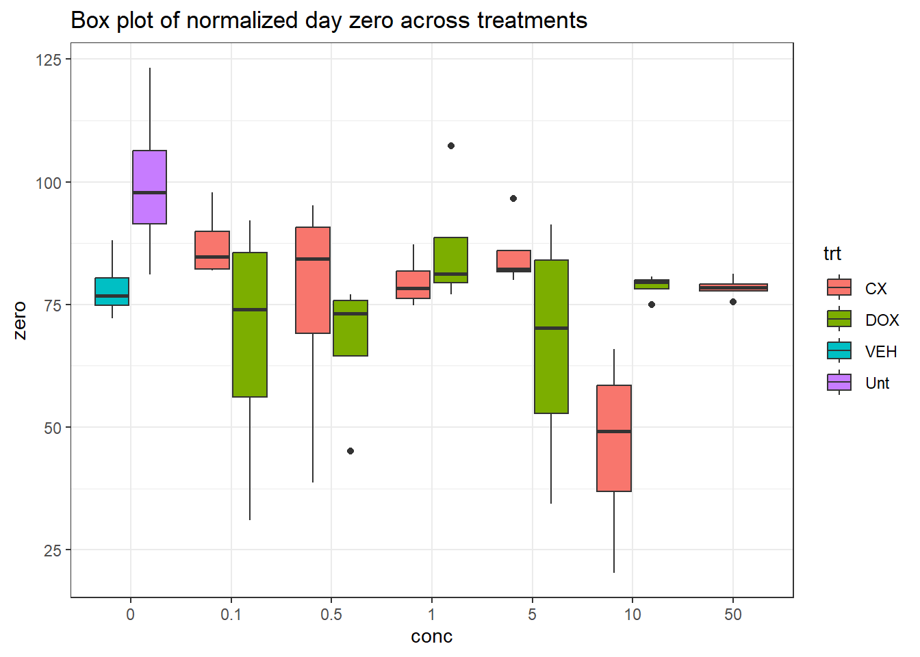

Past versions of plots-1.png

Version	Author	Date
f2ba629	reneeisnowhere	2025-10-31

final_df %>% 
  dplyr::rename("conc"=conc.x) %>% 
  ggplot(., aes(x=conc, y=two_day))+
  geom_boxplot(aes(fill=trt))+
  theme_bw()+
  ggtitle("Box plot of normalized day two across treatments")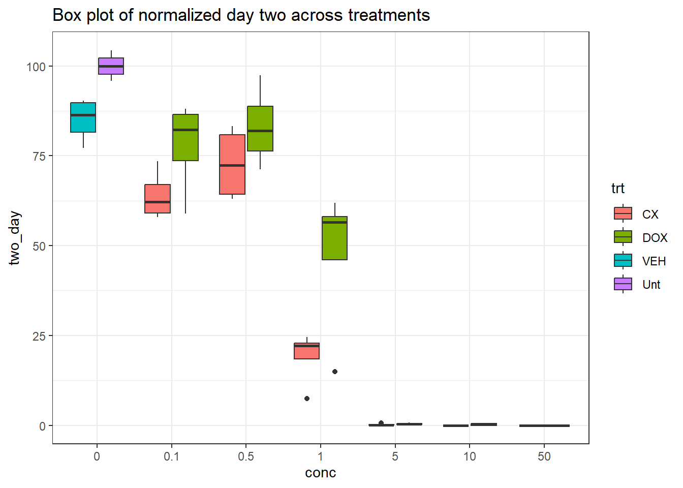

Past versions of plots-2.png

Version	Author	Date
f2ba629	reneeisnowhere	2025-10-31

final_df %>% 
  dplyr::rename("conc"=conc.x) %>% 
  ggplot(., aes(x=conc, y=hr_norm))+
  geom_boxplot(aes(fill=trt))+
  theme_bw()+
  ggtitle("Box plot of normalized across time for each well (between plates)")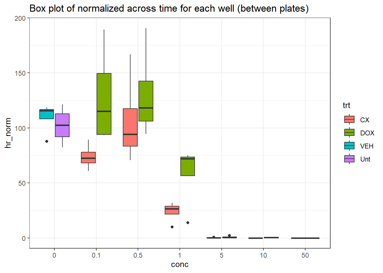

Past versions of plots-3.png

Version	Author	Date
f2ba629	reneeisnowhere	2025-10-31

# Fit
gpt_try <- final_df %>%
  filter(trt == "CX") %>%
  mutate(conc.x = as.numeric(as.character(conc.x))) 
model <- final_df %>%
  filter(trt == "CX") %>%
  mutate(conc.x = as.numeric(as.character(conc.x))) %>% 
  drm(hr_norm ~ conc.x, data = ., fct = L.4())

# Predict across log-spaced range
pred <- data.frame(conc.x = exp(seq(log(min(gpt_try$conc.x[gpt_try$conc.x > 0])),
                                    log(max(gpt_try$conc.x)),
                                    length.out = 100)))
pred$hr_norm <- predict(model, newdata = pred)


LD50 <- ED(model, 50, interval = "delta")  # 50% effective dose

Estimated effective doses

       Estimate Std. Error    Lower    Upper
e:1:50 0.939655   0.077668 0.777642 1.101668

LD50_val <- as.numeric(LD50[1,1])
# Plot
gpt_try %>%
  filter(trt == "CX") %>%
  ggplot(aes(x = conc.x, y = hr_norm)) +
  geom_point() +
  geom_line(data = pred, aes(x = conc.x, y = hr_norm), color = "blue", size = 1) +
  geom_vline(xintercept = LD50_val, color = "red", linetype = "dashed") +
  annotate("text", x = LD50_val, y = max(gpt_try$hr_norm, na.rm = TRUE),
           label = paste0("LD50 = ", signif(LD50_val, 3)),
           color = "red", angle = 90, vjust = -0.5, hjust = 1.1) +
  scale_x_log10() +
  theme_minimal()+
  ggtitle("iPSC 87-1 Dose response Assay for CX")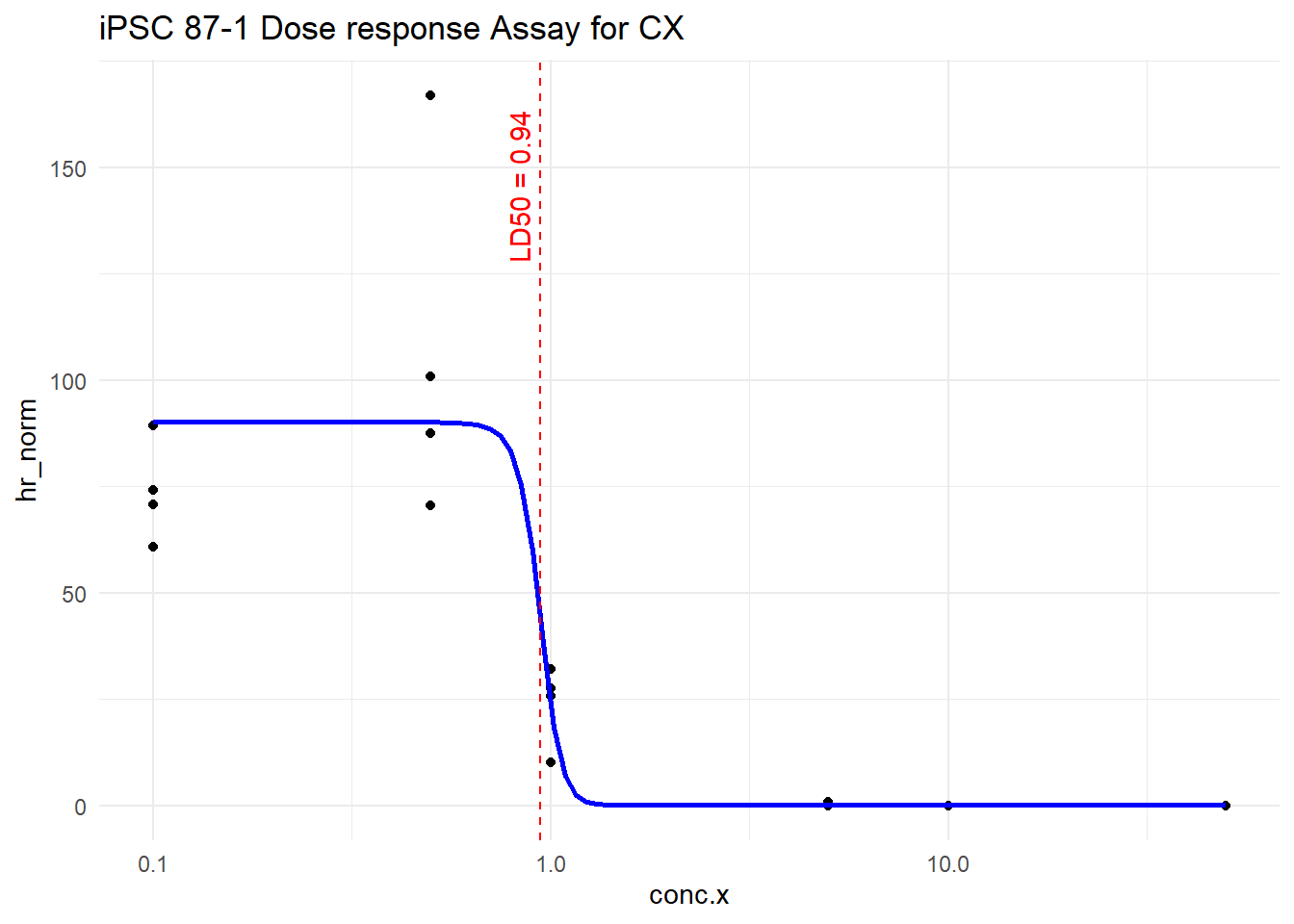

Past versions of "CX DRC first run-1.png"

Version	Author	Date
f2ba629	reneeisnowhere	2025-10-31

# Fit
gpt_try_DOX <- final_df %>%
  filter(trt == "DOX") %>%
  mutate(conc.x = as.numeric(as.character(conc.x))) 
model_DOX <- final_df %>%
  filter(trt == "DOX") %>%
  mutate(conc.x = as.numeric(as.character(conc.x))) %>% 
  drm(hr_norm ~ conc.x, data = ., fct = L.4())

# Predict across log-spaced range
pred_DOX <- data.frame(conc.x = exp(seq(log(min(gpt_try_DOX$conc.x[gpt_try_DOX$conc.x > 0])),
                                    log(max(gpt_try_DOX$conc.x)),
                                    length.out = 100)))
pred_DOX$hr_norm <- predict(model_DOX, newdata = pred_DOX)


LD50_DOX <- ED(model_DOX, 50, interval = "delta")  # 50% effective dose

Estimated effective doses

       Estimate Std. Error   Lower   Upper
e:1:50  0.97482    0.07383 0.81830 1.13133

LD50_val_DOX <- as.numeric(LD50_DOX[1,1])
# Plot
gpt_try_DOX %>%
  filter(trt == "DOX") %>%
  ggplot(aes(x = conc.x, y = hr_norm)) +
  geom_point() +
  geom_line(data = pred_DOX, aes(x = conc.x, y = hr_norm), color = "blue", size = 1) +
  geom_vline(xintercept = LD50_val_DOX, color = "red", linetype = "dashed") +
  annotate("text", x = LD50_val_DOX, y = max(gpt_try_DOX$hr_norm, na.rm = TRUE),
           label = paste0("LD50 = ", signif(LD50_val_DOX, 3)),
           color = "red", angle = 90, vjust = -0.5, hjust = 1.1) +
  scale_x_log10() +
  theme_minimal()+
  ggtitle("iPSC 87-1 Dose response Assay for DOX")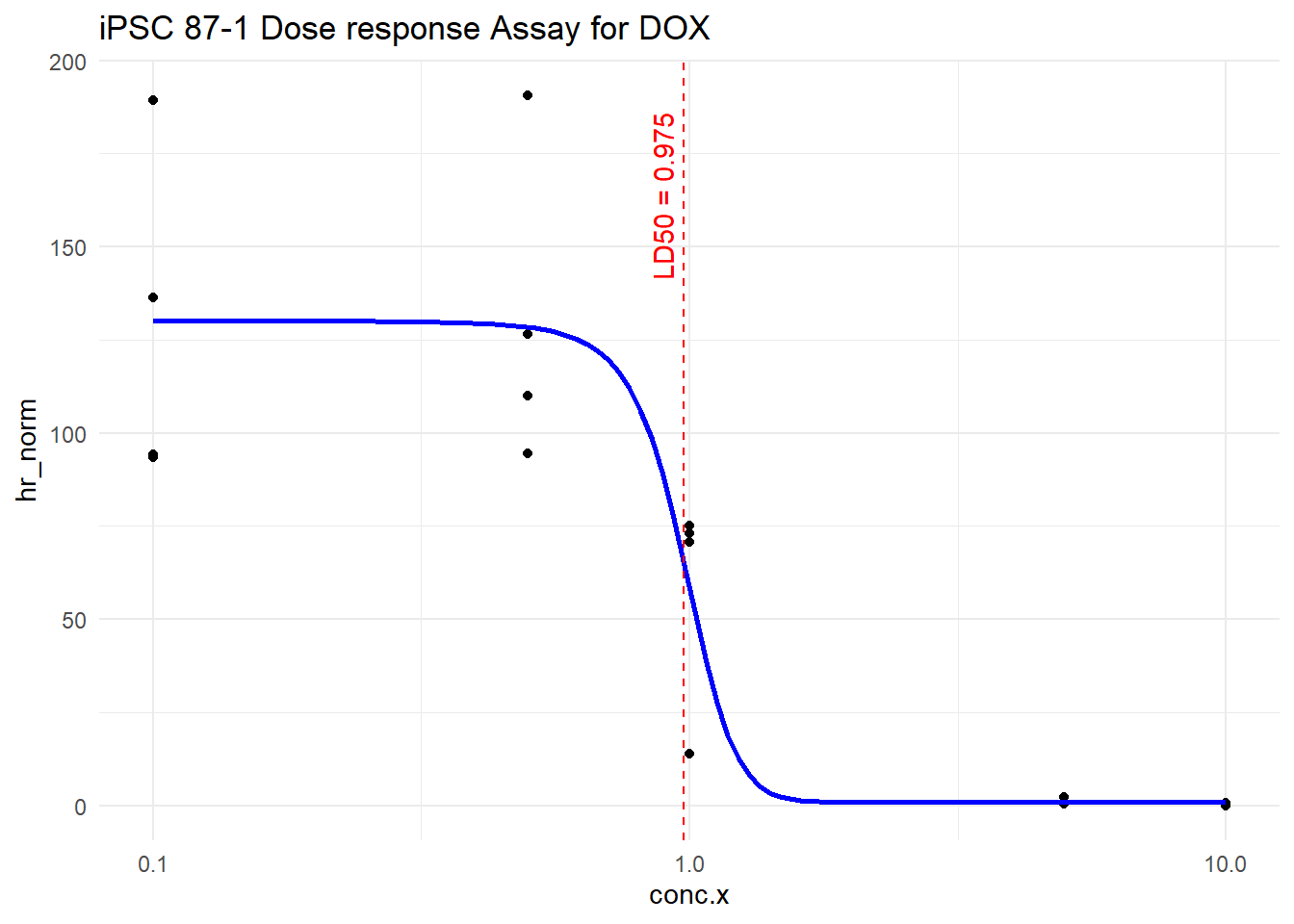

Past versions of "DOX DRC first run-1.png"

Version	Author	Date
f2ba629	reneeisnowhere	2025-10-31

75-1 iPSC renee

T0_75_iPSC_p1_viability <- read_excel("data/Presto_blue_results/75_p1_iPSC_T0_251026.xls", 
    skip = 26)

T0_75_iPSC_p2_viability <- read_excel("data/Presto_blue_results/75_p2_iPSC_T0_251026.xls", 
    skip = 26)

T48_75_iPSC_p1_viability <- read_excel("data/Presto_blue_results/75_iPSC_p1_T48_251028.xlsx", 
    skip = 26)

T48_75_iPSC_p2_viability <- read_excel("data/Presto_blue_results/75_iPSC_p2_T48_251028.xlsx", 
    skip = 26)

iPSC_75_viability_data <- 
T0_75_iPSC_p1_viability %>% 
  mutate(Well="T0_p1") %>% 
  bind_rows(T0_75_iPSC_p2_viability %>% 
              mutate(Well="T0_p2")) %>% 
  bind_rows(T48_75_iPSC_p1_viability %>% 
              mutate(Well="T48_p1")) %>% 
   bind_rows(T48_75_iPSC_p2_viability %>% 
              mutate(Well="T48_p2")) %>% 
  dplyr::rename("Time_Plate"=Well) %>% 
  pivot_longer(., A1:H12, names_to = "Well", values_to = "reading") %>% 
  pivot_wider(id_cols=c("Well"), names_from = "Time_Plate", values_from = "reading")

iPSC_plate_map <- read_excel("data/Presto_blue_results/iPSC_cell_viability_platemap.xlsx", 
    skip = 9)

  base_df_75 <-iPSC_plate_map %>%
  separate(tx_conc, into = c("tx","conc"), sep = "_") %>% 
  left_join(., iPSC_75_viability_data, by = "Well") %>%
    pivot_longer(cols = c(T0_p1, T0_p2, T48_p1,T48_p2), names_to = "Time_plate") %>%
  separate(Time_plate, into = c("Time","plate"), sep = "_") %>% 
  mutate(
    tx  = factor(tx, levels = c("CX", "DOX", "VEH", "untx", "blank")),   # check these levels match your data
    conc = factor(conc, levels = c("0","0.05","0.1","0.5","0.75","1","5","10","na")),
    Time = factor(Time, levels = c("T0","T48"))
  )
  
  # 1. subtract blank per Time and clip negatives
processed_75 <- base_df_75 %>%
  group_by(plate,Time) %>%
  mutate(
    blank_mean = mean(value[tx == "blank"], na.rm = TRUE),
    adj_reading = pmax(value - blank_mean, 0)
  ) %>%
  ungroup()


untx_per_plate_75 <- processed_75 %>%
  filter(tx == "untx") %>%
  group_by(plate, Time) %>%
  summarise(
    untx_mean = mean(adj_reading, na.rm = TRUE),
    n_untx = n(),
    .groups = "drop"
  )



with_untx_75 <- processed_75 %>%
  left_join(untx_per_plate_75, by = c("plate", "Time")) %>%
  mutate(
    norm_to_untx = if_else(
      !is.na(untx_mean) & untx_mean > 0,
      (adj_reading / untx_mean) * 100,
      NA_real_
    )
  ) %>%
  ungroup()


wide_norm_75 <-with_untx_75 %>%
  dplyr::select(Well, tx, conc, Time, plate,norm_to_untx) %>%
  pivot_wider(id_cols = c(Well, tx, conc,plate), names_from = Time, values_from = norm_to_untx)
  
  # Step 5: compute between-time ratio (two_day relative to zero) safely
final_df_75 <- wide_norm_75 %>%
  mutate(
    hr_norm = case_when(
      is.na(T0) | is.na(T48) ~ NA_real_,
      T0 == 0                    ~ NA_real_,   # choose NA to flag unreliable ratio (or 0 if you prefer)
      TRUE                         ~ (T48 / T0) * 100
    )
  ) %>%
  filter(tx != "blank")

final_df_75 %>% 
  # dplyr::rename("conc"=conc.x) %>% 
  ggplot(., aes(x=conc, y=hr_norm))+
  geom_boxplot(aes(fill=tx))+
  theme_bw()+
  facet_wrap(~tx)+
  ggtitle("Box plot of normalized 75 DRC")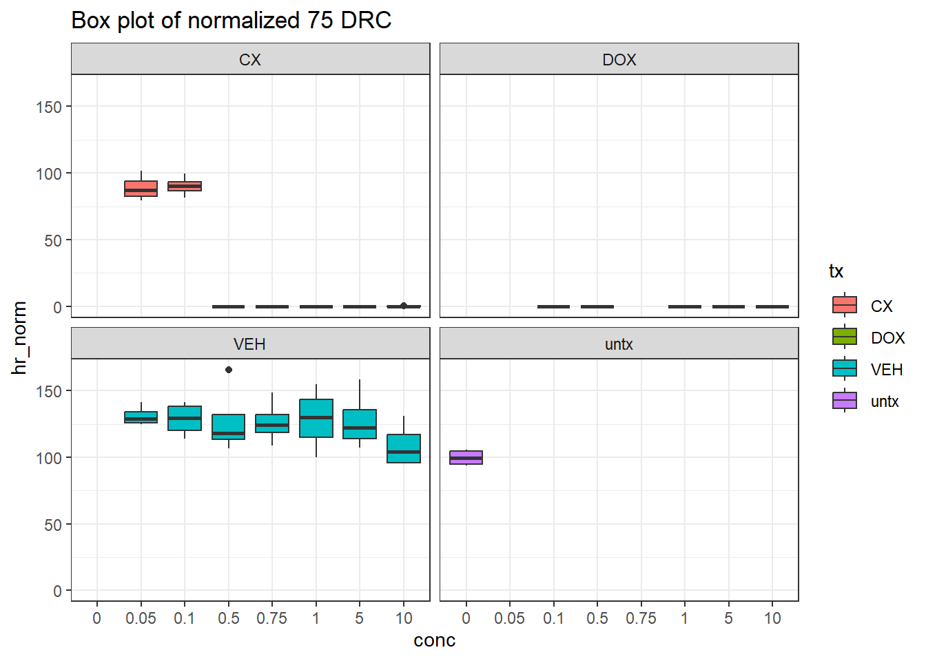

Past versions of "plot 75-1.png"

Version	Author	Date
f2ba629	reneeisnowhere	2025-10-31

78-1 iPSC renee

T0_78_iPSC_p1_viability <- read_excel("data/Presto_blue_results/78_p1_iPSC_T0_251026.xls", 
    skip = 26)

T0_78_iPSC_p2_viability <- read_excel("data/Presto_blue_results/78_p2_iPSC_T0_251026.xls", 
    skip = 26)

T48_78_iPSC_p1_viability <- read_excel("data/Presto_blue_results/78_iPSC_p1_T48_251028.xlsx", 
    skip = 26)

T48_78_iPSC_p2_viability <- read_excel("data/Presto_blue_results/78_iPSC_p2_T48_251028.xlsx", 
    skip = 26)

iPSC_78_viability_data <- 
T0_78_iPSC_p1_viability %>% 
  mutate(Well="T0_p1") %>% 
  bind_rows(T0_78_iPSC_p2_viability %>% 
              mutate(Well="T0_p2")) %>% 
  bind_rows(T48_78_iPSC_p1_viability %>% 
              mutate(Well="T48_p1")) %>% 
   bind_rows(T48_78_iPSC_p2_viability %>% 
              mutate(Well="T48_p2")) %>% 
  dplyr::rename("Time_Plate"=Well) %>% 
  pivot_longer(., A1:H12, names_to = "Well", values_to = "reading") %>% 
  pivot_wider(id_cols=c("Well"), names_from = "Time_Plate", values_from = "reading")

iPSC_plate_map <- read_excel("data/Presto_blue_results/iPSC_cell_viability_platemap.xlsx", 
    skip = 9)

  base_df_78 <-iPSC_plate_map %>%
  separate(tx_conc, into = c("tx","conc"), sep = "_") %>% 
  left_join(., iPSC_78_viability_data, by = "Well") %>%
    pivot_longer(cols = c(T0_p1, T0_p2, T48_p1,T48_p2), names_to = "Time_plate") %>%
  separate(Time_plate, into = c("Time","plate"), sep = "_") %>% 
  mutate(
    tx  = factor(tx, levels = c("CX", "DOX", "VEH", "untx", "blank")),   # check these levels match your data
    conc = factor(conc, levels = c("0","0.05","0.1","0.5","0.75","1","5","10","na")),
    Time = factor(Time, levels = c("T0","T48"))
  )
  
  # 1. subtract blank per Time and clip negatives
processed_78 <- base_df_78 %>%
  group_by(plate,Time) %>%
  mutate(
    blank_mean = mean(value[tx == "blank"], na.rm = TRUE),
    adj_reading = pmax(value - blank_mean, 0)
  ) %>%
  ungroup()


untx_per_plate_78 <- processed_78 %>%
  filter(tx == "untx") %>%
  group_by(plate, Time) %>%
  summarise(
    untx_mean = mean(adj_reading, na.rm = TRUE),
    n_untx = n(),
    .groups = "drop"
  )



with_untx_78 <- processed_78 %>%
  left_join(untx_per_plate_78, by = c("plate", "Time")) %>%
  mutate(
    norm_to_untx = if_else(
      !is.na(untx_mean) & untx_mean > 0,
      (adj_reading / untx_mean) * 100,
      NA_real_
    )
  ) %>%
  ungroup()


wide_norm_78 <-with_untx_78 %>%
  dplyr::select(Well, tx, conc, Time, plate,norm_to_untx) %>%
  pivot_wider(id_cols = c(Well, tx, conc,plate), names_from = Time, values_from = norm_to_untx)
  
  # Step 5: compute between-time ratio (two_day relative to zero) safely
final_df_78 <- wide_norm_78 %>%
  mutate(
    hr_norm = case_when(
      is.na(T0) | is.na(T48) ~ NA_real_,
      T0 == 0                    ~ NA_real_,   # choose NA to flag unreliable ratio (or 0 if you prefer)
      TRUE                         ~ (T48 / T0) * 100
    )
  ) %>%
  filter(tx != "blank")

final_df_78 %>% 
  # dplyr::rename("conc"=conc.x) %>% 
  ggplot(., aes(x=conc, y=hr_norm))+
  geom_boxplot(aes(fill=tx))+
  theme_bw()+
  facet_wrap(~tx)+
  ggtitle("Box plot of normalized 78 DRC")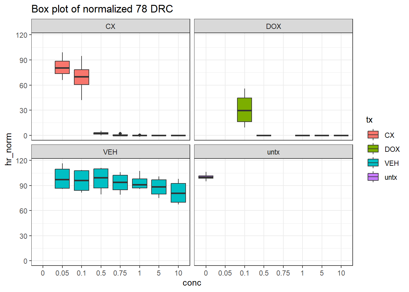

Past versions of "plot 78-1.png"

Version	Author	Date
f2ba629	reneeisnowhere	2025-10-31

87-1 iPSC renee

T0_87_iPSC_p1_viability <- read_excel("data/Presto_blue_results/87_iPSC_p1_T0_251027.xlsx", 
    skip = 26)

T0_87_iPSC_p2_viability <- read_excel("data/Presto_blue_results/87_iPSC_p2_T0_251027.xlsx", 
    skip = 26)

T48_87_iPSC_p1_viability <- read_excel("data/Presto_blue_results/87_iPSC_p1_T48_251029.xlsx", 
    skip = 26)

T48_87_iPSC_p2_viability <- read_excel("data/Presto_blue_results/87_iPSC_p2_T48_251029.xlsx", 
    skip = 26)

iPSC_87_viability_data <- 
T0_87_iPSC_p1_viability %>% 
  mutate(Well="T0_p1") %>% 
  bind_rows(T0_87_iPSC_p2_viability %>% 
              mutate(Well="T0_p2")) %>% 
  bind_rows(T48_87_iPSC_p1_viability %>% 
              mutate(Well="T48_p1")) %>% 
   bind_rows(T48_87_iPSC_p2_viability %>% 
              mutate(Well="T48_p2")) %>% 
  dplyr::rename("Time_Plate"=Well) %>% 
  pivot_longer(., A1:H12, names_to = "Well", values_to = "reading") %>% 
  pivot_wider(id_cols=c("Well"), names_from = "Time_Plate", values_from = "reading")

  base_df_87 <-iPSC_plate_map %>%
  separate(tx_conc, into = c("tx","conc"), sep = "_") %>% 
  left_join(., iPSC_87_viability_data, by = "Well") %>%
    pivot_longer(cols = c(T0_p1, T0_p2, T48_p1,T48_p2), names_to = "Time_plate") %>%
  separate(Time_plate, into = c("Time","plate"), sep = "_") %>% 
  mutate(
    tx  = factor(tx, levels = c("CX", "DOX", "VEH", "untx", "blank")),   # check these levels match your data
    conc = factor(conc, levels = c("0","0.05","0.1","0.5","0.75","1","5","10","na")),
    Time = factor(Time, levels = c("T0","T48"))
  )
  
  # 1. subtract blank per Time and clip negatives
processed_87 <- base_df_87 %>%
  group_by(plate,Time) %>%
  mutate(
    blank_mean = mean(value[tx == "blank"], na.rm = TRUE),
    adj_reading = pmax(value - blank_mean, 0)
  ) %>%
  ungroup()


untx_per_plate_87 <- processed_87 %>%
  filter(tx == "untx") %>%
  group_by(plate, Time) %>%
  summarise(
    untx_mean = mean(adj_reading, na.rm = TRUE),
    n_untx = n(),
    .groups = "drop"
  )



with_untx_87 <- processed_87 %>%
  left_join(untx_per_plate_87, by = c("plate", "Time")) %>%
  mutate(
    norm_to_untx = if_else(
      !is.na(untx_mean) & untx_mean > 0,
      (adj_reading / untx_mean) * 100,
      NA_real_
    )
  ) %>%
  ungroup()


wide_norm_87 <-with_untx_87 %>%
  dplyr::select(Well, tx, conc, Time, plate,norm_to_untx) %>%
  pivot_wider(id_cols = c(Well, tx, conc,plate), names_from = Time, values_from = norm_to_untx)
  
  # Step 5: compute between-time ratio (two_day relative to zero) safely
final_df_87 <- wide_norm_87 %>%
  mutate(
    hr_norm = case_when(
      is.na(T0) | is.na(T48) ~ NA_real_,
      T0 == 0                    ~ NA_real_,   # choose NA to flag unreliable ratio (or 0 if you prefer)
      TRUE                         ~ (T48 / T0) * 100
    )
  ) %>%
  filter(tx != "blank")

final_df_87 %>% 
  # dplyr::rename("conc"=conc.x) %>% 
  ggplot(., aes(x=conc, y=hr_norm))+
  geom_boxplot(aes(fill=tx))+
  theme_bw()+
  facet_wrap(~tx)+
  ggtitle("Box plot of normalized 87 DRC")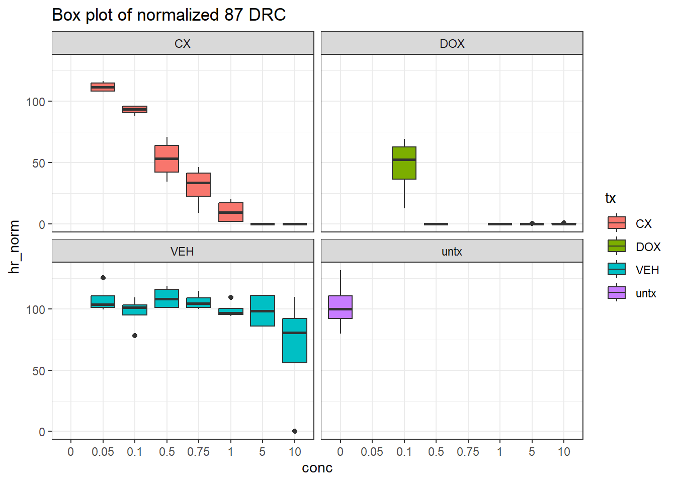

Past versions of "plot 87-1.png"

Version	Author	Date
f2ba629	reneeisnowhere	2025-10-31

plot function

plot_drc <- function(data, tx_name, resp_col = "hr_norm", title = NULL, color_line = "blue") {
  # Filter and prepare data
  df_sub <- data %>%
    filter(tx == tx_name) %>%
    mutate(
      conc = as.numeric(as.character(conc)),
      response = as.numeric(.data[[resp_col]])
    )
  
  # Fit dose-response model
  model <- drm(response ~ conc, data = df_sub, fct = L.4(fixed = c(NA, NA, 100, NA)))
  
  # Generate log-spaced predictions
  pred <- data.frame(conc = exp(seq(
    log(min(df_sub$conc[df_sub$conc > 0], na.rm = TRUE)),
    log(max(df_sub$conc, na.rm = TRUE)),
    length.out = 100
  )))
  pred$response <- predict(model, newdata = pred)
  
  # LD50
  LD50 <- ED(model, 50, interval = "delta")
  LD50_val <- as.numeric(LD50[1, 1])
  
  # Create title if missing
  if (is.null(title)) {
    title <- paste("Dose–Response Curve for", trt_name)
  }
  
  # Plot
  p <- ggplot(df_sub, aes(x = conc, y = response)) +
    geom_point(size = 2, alpha = 0.8) +
    geom_line(data = pred, aes(x = conc, y = response), color = color_line, size = 1) +
    geom_vline(xintercept = LD50_val, color = "red", linetype = "dashed") +
    annotate(
      "text",
      x = LD50_val,
      y = max(df_sub$response, na.rm = TRUE),
      label = paste0("LD50 = ", signif(LD50_val, 3)),
      color = "red", angle = 90, vjust = -0.5, hjust = 1.1
    ) +
    scale_x_log10() +
    theme_minimal(base_size = 14) +
    labs(title = title, x = "Concentration", y = "Response (normalized)")
  
  # Return list so you can use both plot and model
  return(list(plot = p, model = model, LD50 = LD50))
}

All CX plots for iPSCs

CX_75_iPSC <- plot_drc(final_df_75, tx_name = "CX", title = "iPSC 75-1 Dose Response for CX")

Estimated effective doses

       Estimate Std. Error    Lower    Upper
e:1:50 0.196866   0.077915 0.036398 0.357335

CX_75_iPSC$plot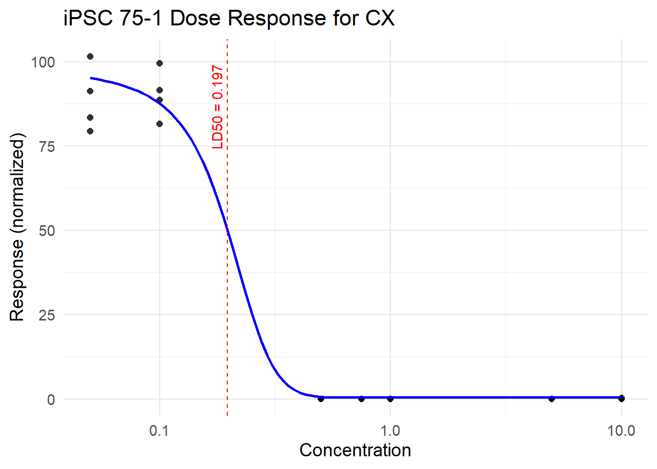

Past versions of unnamed-chunk-2-1.png

Version	Author	Date
f2ba629	reneeisnowhere	2025-10-31

CX_78_iPSC <- plot_drc(final_df_78, tx_name = "CX", title = "iPSC 78-1 Dose Response for CX")

Estimated effective doses

       Estimate Std. Error    Lower    Upper
e:1:50 0.165140   0.044385 0.073727 0.256553

CX_78_iPSC$plot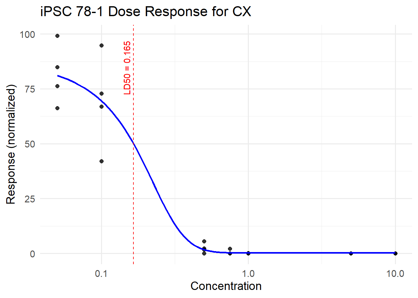

Past versions of unnamed-chunk-2-2.png

Version	Author	Date
f2ba629	reneeisnowhere	2025-10-31

CX_87_iPSC <- plot_drc(final_df_87, tx_name = "CX", title = "iPSC 87-1 Dose Response for CX")

Estimated effective doses

       Estimate Std. Error    Lower    Upper
e:1:50 0.559776   0.040025 0.477168 0.642383

CX_87_iPSC$plot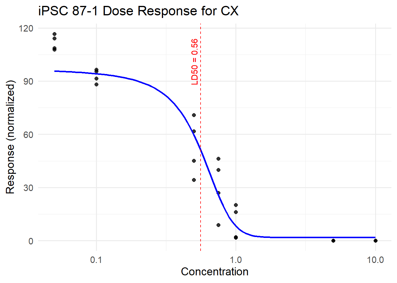

Past versions of unnamed-chunk-2-3.png

Version	Author	Date
f2ba629	reneeisnowhere	2025-10-31

ggplot(
  final_df_78 %>% filter(tx == "CX") %>%
    mutate(conc = as.numeric(as.character(conc))),
  aes(x = conc, y = hr_norm)
) +
  geom_point(size = 2) +
  stat_smooth(
    method = drm,
    method.args = list(fct = L.4(fixed = c(NA, NA, 100, NA))),
    se = FALSE,
    color = "blue"
  ) +
  scale_x_log10() +
  theme_minimal() +
  labs(title = "CX Dose–Response", x = "Concentration", y = "Normalized viability (%)")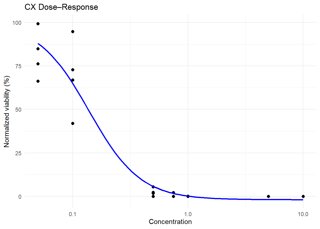

Past versions of unnamed-chunk-3-1.png

Version	Author	Date
f2ba629	reneeisnowhere	2025-10-31

# write_csv(final_df_87,"data/iPSC_87_DRC_20251029.csv")
# write_csv(final_df_75,"data/iPSC_75_DRC_20251028.csv")
# write_csv(final_df_78,"data/iPSC_78_DRC_20251028.csv")

Cardiomyocyte treatment

CM_platemap <- read_excel("data/Presto_blue_results/CM_cell_viability_platemap.xlsx", 
    skip = 9
    )

T0_87_CM_p1_viability <- read_excel("data/Presto_blue_results/87_iPSC-CM_p1_T0_251028.xlsx", 
    skip = 26)

T0_87_CM_p2_viability <- read_excel("data/Presto_blue_results/87_iPSC-CM_p2_T0_251028.xlsx", 
    skip = 26)

T0_87_CM_p3_viability <- read_excel("data/Presto_blue_results/87_iPSC-CM_p3_T0_251028.xlsx", 
    skip = 26)

T0_87_CM_p4_viability <- read_excel("data/Presto_blue_results/87_iPSC-CM_p4_T0_251028.xlsx", 
    skip = 26)
T3_87_CM_p1_viability <- read_excel("data/Presto_blue_results/87_iPSC-CM_p1_T3_251028.xlsx", 
    skip = 26)

T24_87_CM_p2_viability <- read_excel("data/Presto_blue_results/87_iPSC_CM_p2_T24_251029.xlsx", 
    skip = 26)

T48_87_CM_p3_viability <- read_excel("data/Presto_blue_results/87_CM_p3_T48_251030.xlsx", 
    skip = 26)

T96_87_CM_p4_viability <- read_excel("C:/Users/renee/Documents/Ward Lab/CX-revision/Presto Blue results/87_CM_p4_T96_251101.xlsx",
    skip = 26)

CM_combo_87 <- T0_87_CM_p1_viability %>% 
  mutate(Well="T0_p1") %>% 
  bind_rows(T0_87_CM_p2_viability %>% 
              mutate(Well="T0_p2")) %>% 
  bind_rows(T0_87_CM_p3_viability %>% 
              mutate(Well="T0_p3")) %>% 
   bind_rows(T0_87_CM_p4_viability %>% 
              mutate(Well="T0_p4")) %>% 
  bind_rows(T3_87_CM_p1_viability %>% 
              mutate(Well="T3_p1")) %>% 
  bind_rows(T24_87_CM_p2_viability %>% 
              mutate(Well="T24_p2")) %>% 
  bind_rows(T48_87_CM_p3_viability %>%
              mutate(Well="T48_p3")) %>%
     bind_rows(T96_87_CM_p4_viability %>%
              mutate(Well="T96_p4")) %>%
  dplyr::rename("Time_Plate"=Well) %>% 
  pivot_longer(., A1:H12, names_to = "Well", values_to = "reading") %>% 
  pivot_wider(id_cols=c("Well"), names_from = "Time_Plate", values_from = "reading")

T0_78_CM_p1_viability <- read_excel("data/Presto_blue_results/78_iPSC-CM_p1_T0_251028.xlsx", 
    skip = 26)

T0_78_CM_p2_viability <- read_excel("data/Presto_blue_results/78_iPSC-CM_p2_T0_251028.xlsx", 
    skip = 26)

T0_78_CM_p3_viability <- read_excel("data/Presto_blue_results/78_iPSC-CM_p3_T0_251028.xlsx", 
    skip = 26)

T0_78_CM_p4_viability <- read_excel("data/Presto_blue_results/78_iPSC-CM_p4_T0_251028.xlsx", 
    skip = 26)

T3_78_CM_p1_viability <- read_excel("data/Presto_blue_results/78_iPSC-CM_p1_T3_251028.xlsx", 
    skip = 26)

T24_78_CM_p2_viability <- read_excel("data/Presto_blue_results/78_iPSC_CM_p2_T24_251029.xlsx", 
    skip = 26)

T48_78_CM_p3_viability <- read_excel("data/Presto_blue_results/78_CM_p3_T48_251030.xlsx", 
    skip = 26)

T96_78_CM_p4_viability <- read_excel("C:/Users/renee/Documents/Ward Lab/CX-revision/Presto Blue results/78_CM_p4_T96_251101.xlsx",
    skip = 26)


CM_combo_78 <- T0_78_CM_p1_viability %>% 
  mutate(Well="T0_p1") %>% 
  bind_rows(T0_78_CM_p2_viability %>% 
              mutate(Well="T0_p2")) %>% 
  bind_rows(T0_78_CM_p3_viability %>% 
              mutate(Well="T0_p3")) %>% 
   bind_rows(T0_78_CM_p4_viability %>% 
              mutate(Well="T0_p4")) %>% 
  bind_rows(T3_78_CM_p1_viability %>% 
              mutate(Well="T3_p1")) %>% 
  bind_rows(T24_78_CM_p2_viability %>% 
              mutate(Well="T24_p2")) %>% 
  bind_rows(T48_78_CM_p3_viability %>%
              mutate(Well="T48_p3")) %>%
     bind_rows(T96_78_CM_p4_viability %>%
              mutate(Well="T96_p4")) %>%
  dplyr::rename("Time_Plate"=Well) %>% 
  pivot_longer(., A1:H12, names_to = "Well", values_to = "reading") %>% 
  pivot_wider(id_cols=c("Well"), names_from = "Time_Plate", values_from = "reading")

T0_75_CM_p1_viability <- read_excel("data/Presto_blue_results/75_iPSC-CM_p1_T0_251028.xlsx", 
    skip = 26)

T0_75_CM_p2_viability <- read_excel("data/Presto_blue_results/75_iPSC-CM_p2_T0_251028.xlsx", 
    skip = 26)

T0_75_CM_p3_viability <- read_excel("data/Presto_blue_results/75_iPSC-CM_p3_T0_251028.xlsx", 
    skip = 26)


T24_75_CM_p2_viability <- read_excel("data/Presto_blue_results/75_iPSC_CM_p2_T24_251029.xlsx", 
    skip = 26)

T48_75_CM_p3_viability <- read_excel("data/Presto_blue_results/75_CM_p3_T48_251030.xlsx", 
    skip = 26)


CM_combo_75 <- T0_75_CM_p1_viability %>% 
  mutate(Well="T0_p1") %>% 
  bind_rows(T0_75_CM_p2_viability %>% 
              mutate(Well="T0_p2")) %>% 
  bind_rows(T0_75_CM_p3_viability %>% 
              mutate(Well="T0_p3")) %>% 
  # bind_rows(T3_75_CM_p1_viability %>% 
  #             mutate(Well="T3_p1")) %>% 
  bind_rows(T24_75_CM_p2_viability %>% 
              mutate(Well="T24_p2")) %>% 
  bind_rows(T48_75_CM_p3_viability %>%
              mutate(Well="T48_p3")) %>%
  dplyr::rename("Time_Plate"=Well) %>% 
  pivot_longer(., A1:H12, names_to = "Well", values_to = "reading") %>% 
  pivot_wider(id_cols=c("Well"), names_from = "Time_Plate", values_from = "reading")

87 CM

base_df_87_CM <- 
CM_platemap %>%
  separate(col = tx_conc, into = c("tx", "conc"), sep = "_") %>%
  left_join(., CM_combo_87, by = "Well") %>%
    pivot_longer(cols = c(T0_p1:last_col()), names_to = "Time_plate") %>%
  separate(Time_plate, into=c("Time","plate"), sep = "_") %>% 
  mutate(
    tx  = factor(tx, levels = c("CX", "DOX", "VEH", "untx", "blank")),   # check these levels match your data
    conc = factor(conc, levels = c("0","0.1","0.5","2.5","blank")),
    Time = factor(Time, levels = c("T0","T3","T24","T48","T96"))
  )

  # 1. subtract blank per Time and clip negatives
processed_87_CM <- base_df_87_CM %>%
  group_by(plate,Time) %>%
  mutate(
    blank_mean = mean(value[tx == "blank"], na.rm = TRUE),
    adj_reading = pmax(value - blank_mean, 0)
  ) %>%
  ungroup() %>% 
  ##removing a well with no cells
  dplyr::filter(!(plate == 3 & Well == "C7")) %>% 
  dplyr::filter(!(plate == 3 & Well == "C8"))

## calculate untx values to normalize all other wells
untx_per_plate_87_CM <- processed_87_CM %>%
  filter(tx == "untx") %>%
  group_by(plate, Time) %>%
  summarise(
    untx_mean = mean(adj_reading, na.rm = TRUE),
    n_untx = n(),
    .groups = "drop"
  )


### add the untx values in the plate and normalize to untx
with_untx_87_CM <- processed_87_CM %>%
  left_join(untx_per_plate_87_CM, by = c("plate", "Time")) %>%
  mutate(
    norm_to_untx = if_else(
      !is.na(untx_mean) & untx_mean > 0,
      (adj_reading / untx_mean) * 100,
      NA_real_
    )
  ) %>%
  ungroup()

### Filter out blanks and pivot for T0 to T48 normalizing. (probably pivot by plate first to normalize across the times)
norm_Tx_over_T0_87_CM <- with_untx_87_CM %>%
  # Keep only relevant columns
  filter(tx != "blank") %>%
  dplyr::select(Well, tx, conc, Time, plate, norm_to_untx) %>%
  
  # Ensure consistent order of timepoints
  mutate(Time = factor(Time, levels = unique(Time))) %>%
  
  # Pivot wider so each timepoint is its own column
  pivot_wider(
    id_cols = c(Well, tx, conc, plate),
    names_from = Time,
    values_from = norm_to_untx
  ) %>%
  
  # Pivot longer again to calculate T(x)/T0
  pivot_longer(
    cols = -c(Well, tx, conc, plate),
    names_to = "Time",
    values_to = "value"
  ) %>%
  group_by(Well, tx, conc, plate) %>%
  mutate(
    T0_value = value[Time == "T0"],
    Tx_over_T0 = if_else(
      !is.na(T0_value) & T0_value > 0,
      (value / T0_value) * 100,   # convert ratio to percent
      NA_real_
    )
  ) %>%
  ungroup() %>%
  dplyr::select(Well, tx, conc, plate, Time, Tx_over_T0)
# norm_Tx_over_T0_87_CM <-
# with_untx_87_CM %>%
#   filter(tx != "blank") %>%
#   dplyr::select(Well, tx, conc, Time, plate, norm_to_untx) %>%
#   pivot_wider(
#     id_cols = c(Well, tx, conc, plate),
#     names_from = Time,
#     values_from = norm_to_untx
#   ) %>%
#   mutate(
#     norm_T3_T0  = if_else(!is.na(T0) & T0 > 0, T3  / T0, NA_real_),
#     norm_T24_T0 = if_else(!is.na(T0) & T0 > 0, T24 / T0, NA_real_))#,
#     # norm_T48_T0 = if_else(!is.na(T0) & T0 > 0, T48 / T0, NA_real_),
#     # norm_T96_T0 = if_else(!is.na(T0) & T0 > 0, T96 / T0, NA_real_)
#   )
# 
# norm_Tx_over_T0_87_CM_long <- norm_Tx_over_T0_87_CM %>%
#   dplyr::select(Well, tx, conc, plate, starts_with("norm_T")) %>%
#   pivot_longer(
#     cols = starts_with("norm_T"),
#     names_to = "norm_type",
#     values_to = "Tx_over_T0"
#   )

plot 87

norm_Tx_over_T0_87_CM %>% 
  mutate(Time=factor(Time, levels = c("T0", "T3","T24","T48","T96"))) %>% 
  ggplot(aes(x=interaction(tx,conc),y=Tx_over_T0))+
  geom_boxplot(aes(fill=Time))+
  ggtitle("Treatment over time 87")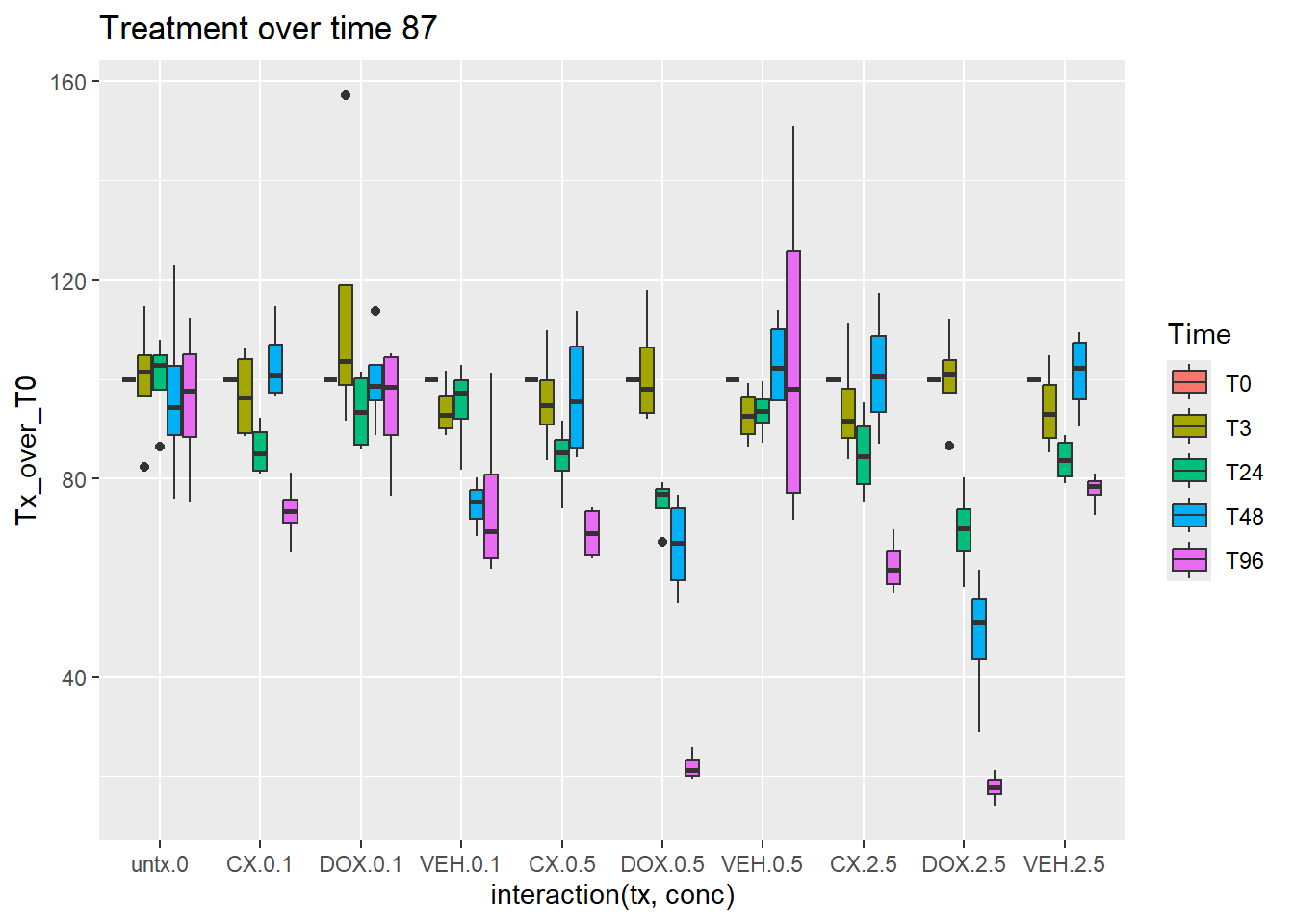

Past versions of unnamed-chunk-5-1.png

Version	Author	Date
f2ba629	reneeisnowhere	2025-10-31

75 CM

base_df_75_CM <- 
CM_platemap %>%
  separate(col = tx_conc, into = c("tx", "conc"), sep = "_") %>%
  left_join(., CM_combo_75, by = "Well") %>%
    pivot_longer(cols = c(T0_p1:last_col()), names_to = "Time_plate") %>%
  separate(Time_plate, into=c("Time","plate"), sep = "_") %>% 
  mutate(
    tx  = factor(tx, levels = c("CX", "DOX", "VEH", "untx", "blank")),   # check these levels match your data
    conc = factor(conc, levels = c("0","0.1","0.5","2.5","blank")),
    Time = factor(Time, levels = c("T0","T3","T24","T48","T96"))
  )

  # 1. subtract blank per Time and clip negatives
processed_75_CM <- base_df_75_CM %>%
  group_by(plate,Time) %>%
  mutate(
    blank_mean = mean(value[tx == "blank"], na.rm = TRUE),
    adj_reading = pmax(value - blank_mean, 0)
  ) %>%
  ungroup()

## calculate untx values to normalize all other wells
untx_per_plate_75_CM <- processed_75_CM %>%
  filter(tx == "untx") %>%
  group_by(plate, Time) %>%
  summarise(
    untx_mean = mean(adj_reading, na.rm = TRUE),
    n_untx = n(),
    .groups = "drop"
  )


### add the untx values in the plate and normalize to untx
with_untx_75_CM <- processed_75_CM %>%
  left_join(untx_per_plate_75_CM, by = c("plate", "Time")) %>%
  mutate(
    norm_to_untx = if_else(
      !is.na(untx_mean) & untx_mean > 0,
      (adj_reading / untx_mean) * 100,
      NA_real_
    )
  ) %>%
  ungroup()

### Filter out blanks and pivot for T0 to T48 normalizing. (probably pivot by plate first to normalize across the times)
norm_Tx_over_T0_75_CM <- with_untx_75_CM %>%
  # Keep only relevant columns
  filter(tx != "blank") %>%
  dplyr::select(Well, tx, conc, Time, plate, norm_to_untx) %>%
  
  # Ensure consistent order of timepoints
  mutate(Time = factor(Time, levels = unique(Time))) %>%
  
  # Pivot wider so each timepoint is its own column
  pivot_wider(
    id_cols = c(Well, tx, conc, plate),
    names_from = Time,
    values_from = norm_to_untx
  ) %>%
  
  # Pivot longer again to calculate T(x)/T0
  pivot_longer(
    cols = -c(Well, tx, conc, plate),
    names_to = "Time",
    values_to = "value"
  ) %>%
  group_by(Well, tx, conc, plate) %>%
  mutate(
    T0_value = value[Time == "T0"],
    Tx_over_T0 = if_else(
      !is.na(T0_value) & T0_value > 0,
      (value / T0_value) * 100,   # convert ratio to percent
      NA_real_
    )
  ) %>%
  ungroup() %>%
  dplyr::select(Well, tx, conc, plate, Time, Tx_over_T0)
# norm_Tx_over_T0_75_CM <-
# with_untx_75_CM %>%
#   filter(tx != "blank") %>%
#   dplyr::select(Well, tx, conc, Time, plate, norm_to_untx) %>%
#   pivot_wider(
#     id_cols = c(Well, tx, conc, plate),
#     names_from = Time,
#     values_from = norm_to_untx
#   ) %>%
#   mutate(
#     norm_T3_T0  = if_else(!is.na(T0) & T0 > 0, T3  / T0, NA_real_),
#     norm_T24_T0 = if_else(!is.na(T0) & T0 > 0, T24 / T0, NA_real_))#,
#     # norm_T48_T0 = if_else(!is.na(T0) & T0 > 0, T48 / T0, NA_real_),
#     # norm_T96_T0 = if_else(!is.na(T0) & T0 > 0, T96 / T0, NA_real_)
#   )
# 
# norm_Tx_over_T0_75_CM_long <- norm_Tx_over_T0_75_CM %>%
#   dplyr::select(Well, tx, conc, plate, starts_with("norm_T")) %>%
#   pivot_longer(
#     cols = starts_with("norm_T"),
#     names_to = "norm_type",
#     values_to = "Tx_over_T0"
#   )

plot 75

norm_Tx_over_T0_75_CM %>% 
  mutate(Time=factor(Time, levels = c("T0", "T3","T24","T48","T96"))) %>% 
  ggplot(aes(x=interaction(tx,conc),y=Tx_over_T0))+
  geom_boxplot(aes(fill=Time))+
  ggtitle("Treatment over time for 75")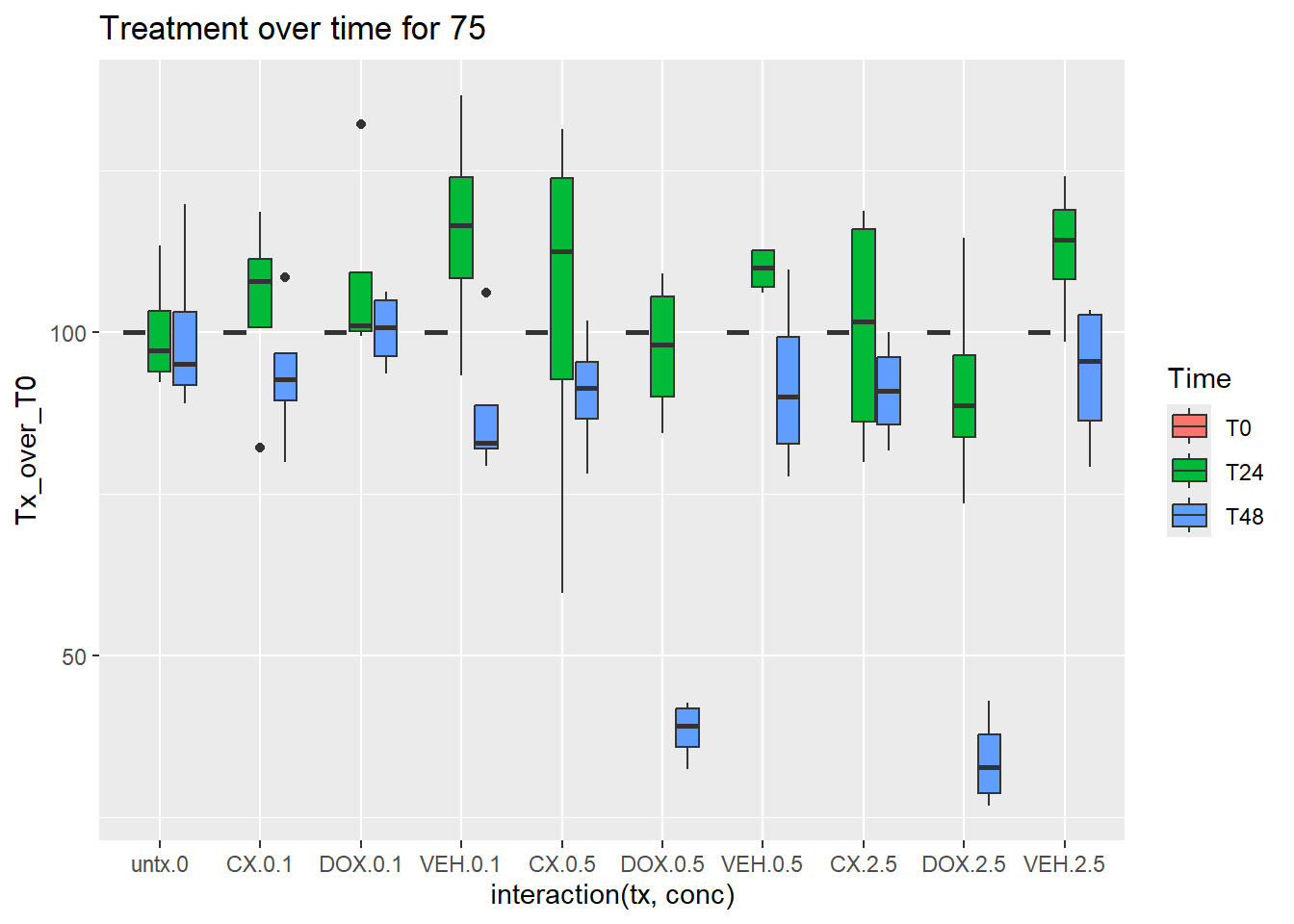

Past versions of unnamed-chunk-6-1.png

Version	Author	Date
f2ba629	reneeisnowhere	2025-10-31

78 CM

base_df_78_CM <- 
CM_platemap %>%
  separate(col = tx_conc, into = c("tx", "conc"), sep = "_") %>%
  left_join(., CM_combo_78, by = "Well") %>%
    pivot_longer(cols = c(T0_p1:last_col()), names_to = "Time_plate") %>%
  separate(Time_plate, into=c("Time","plate"), sep = "_") %>% 
  mutate(
    tx  = factor(tx, levels = c("CX", "DOX", "VEH", "untx", "blank")),   # check these levels match your data
    conc = factor(conc, levels = c("0","0.1","0.5","2.5","blank")),
    Time = factor(Time, levels = c("T0","T3","T24","T48","T96"))
  )

  # 1. subtract blank per Time and clip negatives
processed_78_CM <- base_df_78_CM %>%
  group_by(plate,Time) %>%
  mutate(
    blank_mean = mean(value[tx == "blank"], na.rm = TRUE),
    adj_reading = pmax(value - blank_mean, 0)
  ) %>%
  ungroup()

## calculate untx values to normalize all other wells
untx_per_plate_78_CM <- processed_78_CM %>%
  filter(tx == "untx") %>%
  group_by(plate, Time) %>%
  summarise(
    untx_mean = mean(adj_reading, na.rm = TRUE),
    n_untx = n(),
    .groups = "drop"
  )


### add the untx values in the plate and normalize to untx
with_untx_78_CM <- processed_78_CM %>%
  left_join(untx_per_plate_78_CM, by = c("plate", "Time")) %>%
  mutate(
    norm_to_untx = if_else(
      !is.na(untx_mean) & untx_mean > 0,
      (adj_reading / untx_mean) * 100,
      NA_real_
    )
  ) %>%
  ungroup()

### Filter out blanks and pivot for T0 to T48 normalizing. (probably pivot by plate first to normalize across the times)
norm_Tx_over_T0_78_CM <- with_untx_78_CM %>%
  # Keep only relevant columns
  filter(tx != "blank") %>%
  dplyr::select(Well, tx, conc, Time, plate, norm_to_untx) %>%
  
  # Ensure consistent order of timepoints
  mutate(Time = factor(Time, levels = c("T0","T3","T24","T48","T96"))) %>%
  
  # Pivot wider so each timepoint is its own column
  pivot_wider(
    id_cols = c(Well, tx, conc, plate),
    names_from = Time,
    values_from = norm_to_untx
  ) %>%
  
  # Pivot longer again to calculate T(x)/T0
  pivot_longer(
    cols = -c(Well, tx, conc, plate),
    names_to = "Time",
    values_to = "value"
  ) %>%
  group_by(Well, tx, conc, plate) %>%
  mutate(
    T0_value = value[Time == "T0"],
    Tx_over_T0 = if_else(
      !is.na(T0_value) & T0_value > 0,
      (value / T0_value) * 100,   # convert ratio to percent
      NA_real_
    )
  ) %>%
  ungroup() %>%
  dplyr::select(Well, tx, conc, plate, Time, Tx_over_T0)

plot 78

norm_Tx_over_T0_78_CM %>% 
  mutate(Time=factor(Time, levels = c("T0", "T3","T24","T48","T96"))) %>% 
  ggplot(aes(x=interaction(tx,conc),y=Tx_over_T0))+
  geom_boxplot(aes(fill=Time))+
  ggtitle("Treatment over time for 78")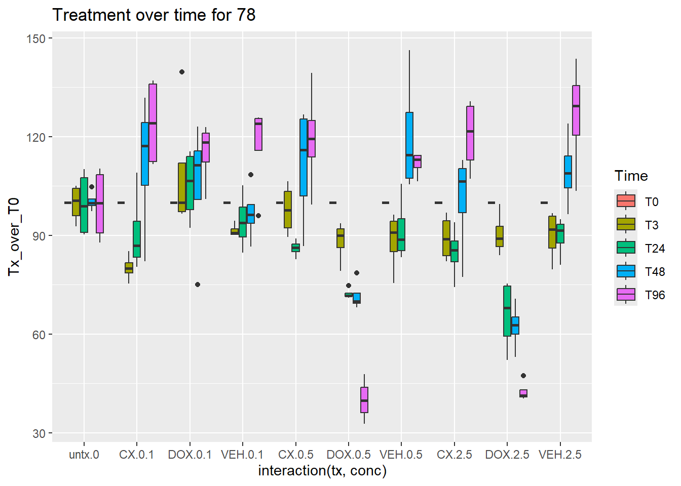

Past versions of unnamed-chunk-7-1.png

Version	Author	Date
f2ba629	reneeisnowhere	2025-10-31

all_lines <- bind_rows(
  norm_Tx_over_T0_87_CM %>% mutate(cell_line = "87"),
  norm_Tx_over_T0_75_CM %>% mutate(cell_line = "75"),
  norm_Tx_over_T0_78_CM %>% mutate(cell_line = "78")
)
summ_all <- all_lines %>%
  group_by(cell_line, tx, conc, Time) %>%
  summarise(
    mean_Tx_over_T0 = mean(Tx_over_T0, na.rm = TRUE),
    se_Tx_over_T0 = sd(Tx_over_T0, na.rm = TRUE) / sqrt(n()),
    .groups = "drop"
  )

All normalized to untx plot

summ_all %>% 
  dplyr::filter(tx %in% c("CX","DOX")) %>% 
  mutate(Time=factor(Time, levels=c("T0","T3","T24","T48","T96")),
         group=paste0(conc,"_",tx)) %>%
  ggplot(aes(x=group,y=mean_Tx_over_T0))+
  geom_boxplot(aes(fill=Time))+
  theme_classic()+
  ggtitle("Treatment over time for all lines just to untx")+
  coord_cartesian(ylim = c(0,115))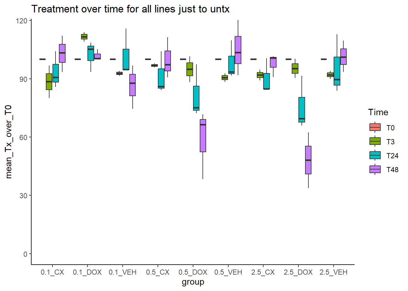

Past versions of "plot all-1.png"

Version	Author	Date
10b921a	reneeisnowhere	2025-10-31
f2ba629	reneeisnowhere	2025-10-31

# write.csv(summ_all,"data/CM_cell_viability_3-96.csv")
# write.csv(all_lines,"data/individual_data_points_CM_cell_viability_3-96.csv")

Normalizing to VEH too

normalize_to_vehicle <- function(platemap_df, combo_df) {
  
  base_df <- platemap_df %>%
    separate(col = tx_conc, into = c("tx", "conc"), sep = "_") %>%
    left_join(., combo_df, by = "Well") %>%
    pivot_longer(cols = c(T0_p1:last_col()), names_to = "Time_plate") %>%
    separate(Time_plate, into = c("Time", "plate"), sep = "_") %>%
    mutate(
      tx = factor(tx, levels = c("CX", "DOX", "VEH", "untx", "blank")),
      conc = factor(conc, levels = c("0","0.1","0.5","2.5","blank")),
      Time = factor(Time, levels = c("T0", "T3", "T24", "T48", "T96"))
    )
  
  # 1️⃣ Subtract blank per Time and clip negatives
  processed <- base_df %>%
    group_by(plate, Time) %>%
    mutate(
      blank_mean = mean(value[tx == "blank"], na.rm = TRUE),
      adj_reading = pmax(value - blank_mean, 0)
    ) %>%
    ungroup()
  
  # 2️⃣ Compute VEH means per plate/time/concentration
  veh_per_plate <- processed %>%
    dplyr::filter(tx == "VEH") %>%
    group_by(plate, Time, conc) %>%
    summarise(
      veh_mean = mean(adj_reading, na.rm = TRUE),
      n_veh = n(),
      .groups = "drop"
    )
  
  # 3️⃣ Join VEH means to all wells & normalize
  with_veh <- processed %>%
    left_join(veh_per_plate, by = c("plate", "Time", "conc")) %>%
    mutate(
      norm_to_veh = if_else(
        !is.na(veh_mean) & veh_mean > 0,
        (adj_reading / veh_mean) * 100,
        NA_real_
      )
    ) %>%
    ungroup()
  
  # 4️⃣ Normalize each timepoint to T0 (Tx/T0)
  norm_Tx_over_T0 <- with_veh %>%
    dplyr::filter(tx != "blank") %>%
    dplyr::select(Well, tx, conc, Time, plate, norm_to_veh) %>%
    mutate(Time = factor(Time, levels = c("T0", "T3", "T24", "T48"))) %>%
    pivot_wider(
      id_cols = c(Well, tx, conc, plate),
      names_from = Time,
      values_from = norm_to_veh
    ) %>%
    pivot_longer(
      cols = -c(Well, tx, conc, plate),
      names_to = "Time",
      values_to = "value"
    ) %>%
    group_by(Well, tx, conc, plate) %>%
    mutate(
      T0_value = value[Time == "T0"],
      Tx_over_T0 = if_else(
        !is.na(T0_value) & T0_value > 0,
        (value / T0_value) * 100,
        NA_real_
      )
    ) %>%
    ungroup() %>%
    dplyr::select(Well, tx, conc, plate, Time, Tx_over_T0)
  
  return(norm_Tx_over_T0)
}

VEH_norm_plot_CM_75 <- normalize_to_vehicle(CM_platemap,CM_combo_75)

VEH_norm_plot_CM_78 <- normalize_to_vehicle(CM_platemap,CM_combo_78)

VEH_norm_plot_CM_87 <- normalize_to_vehicle(CM_platemap,CM_combo_87)

VEH normed plot

all_lines_VEH_norm <- bind_rows(
  VEH_norm_plot_CM_87 %>% mutate(cell_line = "87"),
  VEH_norm_plot_CM_75 %>% mutate(cell_line = "75"),
  VEH_norm_plot_CM_78 %>% mutate(cell_line = "78")
)
summ_all_VEH_norm <- all_lines_VEH_norm %>%
  group_by(cell_line, tx, conc, Time) %>%
  summarise(
    mean_Tx_over_T0 = mean(Tx_over_T0, na.rm = TRUE),
    se_Tx_over_T0 = sd(Tx_over_T0, na.rm = TRUE) / sqrt(n()),
    .groups = "drop"
  )

summ_all_VEH_norm %>% 
  dplyr::filter(tx %in% c("CX","DOX","VEH")) %>% 
  mutate(Time=factor(Time, levels=c("T0","T3","T24","T48")),
         group=paste0(conc,"_",tx)) %>%
  ggplot(aes(x=group,y=mean_Tx_over_T0))+
  geom_boxplot(aes(fill=Time))+
  theme_classic()+
  ggtitle("Treatment over time for all lines VEH norm")+
  coord_cartesian(ylim = c(0,125))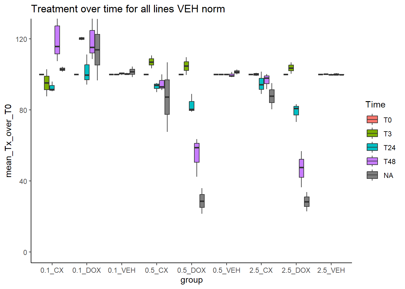

Past versions of "plot all VEH norm-1.png"

Version	Author	Date
f2ba629	reneeisnowhere	2025-10-31

Session information

sessionInfo()

R version 4.4.2 (2024-10-31 ucrt)
Platform: x86_64-w64-mingw32/x64
Running under: Windows 11 x64 (build 26100)

Matrix products: default


locale:
[1] LC_COLLATE=English_United States.utf8 
[2] LC_CTYPE=English_United States.utf8   
[3] LC_MONETARY=English_United States.utf8
[4] LC_NUMERIC=C                          
[5] LC_TIME=English_United States.utf8    

time zone: America/Chicago
tzcode source: internal

attached base packages:
[1] stats     graphics  grDevices utils     datasets  methods   base     

other attached packages:
 [1] drc_3.0-1       MASS_7.3-65     readxl_1.4.5    lubridate_1.9.4
 [5] forcats_1.0.0   stringr_1.5.1   dplyr_1.1.4     purrr_1.1.0    
 [9] readr_2.1.5     tidyr_1.3.1     tibble_3.3.0    ggplot2_3.5.2  
[13] tidyverse_2.0.0 workflowr_1.7.1

loaded via a namespace (and not attached):
 [1] gtable_0.3.6       xfun_0.52          bslib_0.9.0        processx_3.8.6    
 [5] lattice_0.22-7     callr_3.7.6        tzdb_0.5.0         vctrs_0.6.5       
 [9] tools_4.4.2        ps_1.9.1           generics_0.1.4     sandwich_3.1-1    
[13] pkgconfig_2.0.3    Matrix_1.7-3       RColorBrewer_1.1-3 lifecycle_1.0.4   
[17] compiler_4.4.2     farver_2.1.2       git2r_0.36.2       codetools_0.2-20  
[21] getPass_0.2-4      carData_3.0-5      httpuv_1.6.16      htmltools_0.5.8.1 
[25] sass_0.4.10        yaml_2.3.10        Formula_1.2-5      later_1.4.2       
[29] pillar_1.11.0      car_3.1-3          jquerylib_0.1.4    whisker_0.4.1     
[33] cachem_1.1.0       abind_1.4-8        multcomp_1.4-28    nlme_3.1-168      
[37] gtools_3.9.5       tidyselect_1.2.1   digest_0.6.37      mvtnorm_1.3-3     
[41] stringi_1.8.7      labeling_0.4.3     splines_4.4.2      rprojroot_2.1.1   
[45] fastmap_1.2.0      grid_4.4.2         cli_3.6.5          magrittr_2.0.3    
[49] survival_3.8-3     dichromat_2.0-0.1  TH.data_1.1-4      withr_3.0.2       
[53] scales_1.4.0       promises_1.3.3     plotrix_3.8-4      timechange_0.3.0  
[57] rmarkdown_2.29     httr_1.4.7         cellranger_1.1.0   zoo_1.8-14        
[61] hms_1.1.3          evaluate_1.0.5     knitr_1.50         mgcv_1.9-3        
[65] rlang_1.1.6        Rcpp_1.1.0         glue_1.8.0         rstudioapi_0.17.1 
[69] jsonlite_2.0.0     R6_2.6.1           fs_1.6.6